Data Mining (79 page)
Authors: Mehmed Kantardzic

The reader may check that the result of the incremental-clustering process will not be the same if the order of the samples is different. Usually, this algorithm is not iterative (although it could be) and the clusters generated after all the samples have been analyzed in one iteration are the final clusters. If the iterative approach is used, the centroids of the clusters computed in the previous iteration are used as a basis for the partitioning of samples in the next iteration.
For most partitional-clustering algorithms, including the iterative approach, a summarized representation of the cluster is given through its clustering feature (CF) vector. This vector of parameters is given for every cluster as a triple, consisting of the number of points (samples) of the cluster, the centroid of the cluster, and the radius of the cluster. The cluster’s radius is defined as the square-root of the average mean-squared distance from the centroid to the points in the cluster (averaged within-cluster variation). When a new point is added or removed from a cluster, the new CF can be computed from the old CF. It is very important that we do not need the set of points in the cluster to compute a new CF.
If samples are with categorical data, then we do not have a method to calculate centroids as representatives of the clusters. In that case, an additional algorithm called
K-nearest neighbor
may be used to estimate distances (or similarities) between samples and existing clusters. The basic steps of the algorithm are
1.
to compute the distances between the new sample and all previous samples, already classified into clusters;
2.
to sort the distances in increasing order and select K samples with the smallest distance values; and
3.
to apply the voting principle. A new sample will be added (classified) to the largest cluster out of K selected samples.
For example, given six 6-D categorical samples


they are gathered into two clusters C
1
= {X
1
, X
2
, X
3
} and C
2
= {X
4
, X
5
, X
6
}. How does one classify the new sample Y = {A, C, A, B, C, A}?
To apply the K-nearest neighbor algorithm, it is necessary, as the first step, to find all distances between the new sample and the other samples already clustered. Using the SMC measure, we can find similarities instead of distances between samples.
| Similarities with Elements in C 1 | Similarities with Elements in C 2 |
| SMC(Y, X 1 ) = 4/6 = 0.66 | SMC(Y, X 4 ) = 4/6 = 0.66 |
| SMC(Y, X 2 ) = 3/6 = 0.50 | SMC(Y, X 5 ) = 2/6 = 0.33 |
| SMC(Y, X 3 ) = 2/6 = 0.33 | SMC(Y, X 6 ) = 2/6 = 0.33 |
Using the 1-nearest neighbor rule (K = 1), the new sample cannot be classified because there are two samples (X
1
and X
4
) with the same, highest similarity (smallest distances), and one of them is in the class C
1
and the other in the class C
2
. On the other hand, using the 3-nearest neighbor rule (K = 3) and selecting the three largest similarities in the set, we can see that two samples (X
1
and X
2
) belong to class C
1
, and only one sample to class C
2
. Therefore, using a simple voting system we can classify the new sample Y into the C
1
class.
9.6 DBSCAN ALGORITHM
Density-based approach in clustering assumes that clusters are regarded as dense regions of objects in the data space that are separated by regions of low object density (noise). These regions may have an arbitrary shape. Crucial concepts of this approach are density and connectivity both measured in terms of local distribution of nearest neighbors. The algorithm DBSCAN targeting low-dimensional data is the major representative in this category of density-based clustering algorithms. The main reason why DBSCAN recognizes the clusters is that within each cluster we have a typical density of points that is considerably higher than outside of the cluster. Furthermore, the points’ density within the areas of noise is lower than the density in any of the clusters.
DBSCAN is based on two main concepts:
density reachability
and
density connectability
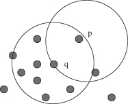
. These both concepts depend on two input parameters of the DBSCAN clustering: the size of epsilon neighborhood (ε) and the minimum points in a cluster (m). The key idea of the DBSCAN algorithm is that, for each point of a cluster, the neighborhood of a given radius ε has to contain at least a minimum number of points m, that is, the density in the neighborhood has to exceed some predefined threshold. For example, in Figure
9.9
point p has only two points in the neighborhood ε, while point q has eight. Obviously, the density around q is higher then around p.
Figure 9.9.
Neighborhood (ε) for points p and q.

Density reachability
defines whether two close points belong to the same cluster. Point p
1
is density-reachable from p
2
if two conditions are satisfied: (1) the points are close enough to each other: distance (p
1
,p
2
) < ε, and (2) there are enough of points in ε neighborhood of p
2
: distance(r,p
2
) > m, where r are some database points. In the example represented in Figure
9.9
, point p is reachable from point q.
Density connectivity
is the next building step of DBSCAN. Points p
0
and p
n
are
density connected
, if there is a sequence of
density-reachable
points (p
0
, p
1
, p
2
, … ) from p
0
to p
n
such that p
i+1
is
density-reachable
from p
i
. These ideas are translated into DBSCAN
cluster
as a set of all density connected points.
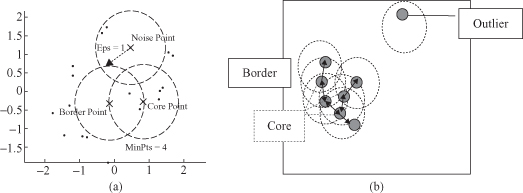
The clustering process is based on the classification of the points in the dataset as
core points
,
border points
, and
noise points
(examples are given in Fig.
9.10
):
- A point is a
core point
if it has more than a specified number of points (m) within neighborhood ε. These are points that are at the interior of a cluster - A
border point
has fewer than m points within its neighborhood ε, but it is in the neighbor of a core point. - A
noise point
is any point that is not a core point or a border point.
Figure 9.10.
Examples of core, border, and noise points. (a) ε and m determine the type of the point; (b) core points build dense regions.

