Structure and Interpretation of Computer Programs (15 page)
Read Structure and Interpretation of Computer Programs Online
Authors: Harold Abelson and Gerald Jay Sussman with Julie Sussman

(define (search f neg-point pos-point)
(let ((midpoint (average neg-point pos-point)))
(if (close-enough? neg-point pos-point)
midpoint
(let ((test-value (f midpoint)))
(cond ((positive? test-value)
(search f neg-point midpoint))
((negative? test-value)
(search f midpoint pos-point))
(else midpoint))))))
We assume that we are initially given the function
f
together with
points at which its values are negative and positive. We first
compute the midpoint of the two given points. Next we check to see if
the given interval is small enough, and if so we simply return the
midpoint as our answer. Otherwise, we compute as a test value the
value of
f
at the midpoint. If the test value is positive, then
we continue the process with a new interval running from the original
negative point to the midpoint. If the test value is negative, we
continue with the interval from the midpoint to the positive point.
Finally, there is the possibility that the test value is 0, in which
case the midpoint is itself the root we are searching for.
To test whether the endpoints are “close enough” we can use a
procedure similar to the one used in section
1.1.7
for
computing square roots:
55
(define (close-enough? x y)
(< (abs (- x y)) 0.001))
Search
is awkward to use directly, because
we can accidentally give it points at which
f
's
values do not have the required sign, in which case we get a wrong answer.
Instead we will use
search
via the following procedure, which
checks to see which of the endpoints has a negative function value and
which has a positive value, and calls the
search
procedure
accordingly. If the function has the same sign on the two given
points, the half-interval method cannot be used, in which case the
procedure signals an error.
56
(define (half-interval-method f a b)
(let ((a-value (f a))
(b-value (f b)))
(cond ((and (negative? a-value) (positive? b-value))
(search f a b))
((and (negative? b-value) (positive? a-value))
(search f b a))
(else
(error "Values are not of opposite sign" a b)))))
The following example uses the half-interval method to approximate π
as the root between 2 and 4 of
sin
x
= 0:
(half-interval-method sin 2.0 4.0)
3.14111328125
Here is another example, using the half-interval method
to search for a root of the equation
x
3
- 2
x
- 3 = 0
between 1 and 2:
(half-interval-method (lambda (x) (- (* x x x) (* 2 x) 3))
1.0
2.0)
1.89306640625
A number
x
is called a
fixed point
of a function
f
if
x
satisfies the equation
f
(
x
) =
x
. For some functions
f
we can locate
a fixed point by beginning with an initial guess and applying
f
repeatedly,

until the value does not change very much. Using this idea, we can
devise a procedure
fixed-point
that takes as inputs a function
and an initial guess and produces an approximation to a fixed point of
the function. We apply the function repeatedly until we find two
successive values whose difference is less than some prescribed
tolerance:
(define tolerance 0.00001)
(define (fixed-point f first-guess)
(define (close-enough? v1 v2)
(< (abs (- v1 v2)) tolerance))
(define (try guess)
(let ((next (f guess)))
(if (close-enough? guess next)
next
(try next))))
(try first-guess))
For example, we can use this method to approximate the fixed point of
the cosine function, starting with 1 as an initial approximation:
57
(fixed-point cos 1.0)
.7390822985224023
Similarly, we can find a solution to the equation
y
=
sin
y
+
cos
y
:
(fixed-point (lambda (y) (+ (sin y) (cos y)))
1.0)
1.2587315962971173
The fixed-point process is reminiscent of the process we used for
finding square roots in section
1.1.7
. Both are based on the
idea of repeatedly improving a guess until the result satisfies some
criterion. In fact, we can readily formulate the
square-root
computation as a fixed-point search. Computing the square root of
some number
x
requires finding a
y
such that
y
2
=
x
. Putting
this equation into the equivalent form
y
=
x
/
y
, we recognize that we
are looking for a fixed point of the function
58
y
⟼
x
/
y
, and we
can therefore try to compute square roots as
(define (sqrt x)
(fixed-point (lambda (y) (/ x y))
1.0))
Unfortunately, this fixed-point search does not converge. Consider an
initial guess
y
1
. The next guess is
y
2
=
x
/
y
1
and the next
guess is
y
3
=
x
/
y
2
=
x
/(
x
/
y
1
) =
y
1
. This results in an infinite
loop in which the two guesses
y
1
and
y
2
repeat over and over,
oscillating about the answer.
One way to control such oscillations is to prevent the guesses from
changing so much.
Since the answer is always between our guess
y
and
x
/
y
, we can make a new guess that is not as far from
y
as
x
/
y
by averaging
y
with
x
/
y
, so that the next guess after
y
is (1/2)(
y
+
x
/
y
) instead of
x
/
y
.
The process of making such a sequence of guesses is simply the process
of looking for a fixed point of
y
⟼ (1/2)(
y
+
x
/
y
):
(define (sqrt x)
(fixed-point (lambda (y) (average y (/ x y)))
1.0))
(Note that
y
= (1/2)(
y
+
x
/
y
) is a simple transformation of the
equation
y
=
x
/
y
; to derive it, add
y
to both sides of the equation
and divide by 2.)
With this modification, the square-root procedure works. In fact, if
we unravel the definitions, we can see that the sequence of
approximations to the square root generated here is precisely the
same as the one generated by our original square-root procedure of
section
1.1.7
. This approach of averaging
successive approximations to a solution, a technique we that we call
average damping
, often aids the convergence of fixed-point
searches.
Exercise 1.35.
Show that the golden ratio
φ
(section
1.2.2
)
is a fixed point of the transformation
x
⟼ 1 + 1/
x
, and use
this fact to compute
φ
by means of the
fixed-point
procedure.
Exercise 1.36.
Modify
fixed-point
so that it prints the sequence of
approximations it generates, using
the
newline
and
display
primitives shown in
exercise
1.22
. Then find a solution to
x
x
=
1000 by finding a fixed point of
x
⟼
log
(1000)/
log
(
x
). (Use
Scheme's
primitive
log
procedure, which computes natural
logarithms.) Compare the number of steps this takes with and without
average damping. (Note that you cannot start
fixed-point
with a
guess of 1, as this would cause division by
log
(1) = 0.)
Exercise 1.37.
a. An infinite
continued fraction
is an expression of the form
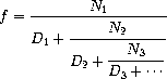
As an example, one can show that the infinite continued fraction
expansion with the
N
i
and the
D
i
all equal to 1 produces
1/
φ
, where
φ
is the golden ratio (described in
section
1.2.2
).
One way to approximate an
infinite continued fraction is to truncate the expansion after a given
number of terms. Such a truncation – a so-called
k
-term finite
continued fraction
– has the form

Suppose that
n
and
d
are procedures of one argument (the
term index
i
) that return the
N
i
and
D
i
of the terms of the
continued fraction. Define a procedure
cont-frac
such that evaluating
(cont-frac n d k)
computes the value of the
k
-term finite
continued fraction. Check your procedure by approximating 1/
φ
using
(cont-frac (lambda (i) 1.0)
(lambda (i) 1.0)
k)
for successive values of
k
. How large must you make
k
in order to get an approximation that is accurate to 4 decimal places?
b. If your
cont-frac
procedure generates a recursive process, write one that generates
an iterative process.
If it generates an iterative process, write one that generates
a recursive process.
Exercise 1.38.
In 1737, the Swiss mathematician Leonhard Euler published a memoir
De Fractionibus Continuis
, which included a
continued fraction
expansion for
e
- 2, where
e
is the base of the natural logarithms.
In this fraction, the
N
i
are all 1, and the
D
i
are successively
1, 2, 1, 1, 4, 1, 1, 6, 1, 1, 8,
...
. Write a program that uses
your
cont-frac
procedure from
exercise
1.37
to approximate
e
, based on
Euler's expansion.