Understanding Computation (11 page)

It’s convenient to be able to parse
Simple
programs like
this, but Treetop is doing all the hard work for us, so we haven’t learned much about how a
parser actually works. In
Parsing with Pushdown Automata
, we’ll see how to implement a
parser
directly.
[
2
]
In the context of programming language theory, the word
semantics
is usually treated as singular: we describe the
meaning of a language by giving it
a semantics
.
[
3
]
Although access to ISO/IEC 30170 costs money, an earlier draft
of the same specification can be downloaded for free from
http://www.ipa.go.jp/osc/english/ruby/
.
[
4
]
This can be an
abbreviation for simple imperative language if you want it to be.
[
5
]
For the sake of simplicity, we’ll resist the urge to extract common code into
superclasses or modules.
[
6
]
Although this is pretty much exactly how we’d write#reducible?in a functional language
like Haskell or ML.
[
7
]
At the moment, it doesn’t make any difference
which
order we
choose, but we can’t avoid making the decision.
[
8
]
This conditional is not the same as Ruby’sif.
In Ruby,ifis an expression that returns a value,
but in
Simple
, it’s a statement for choosing which
of two other statements to evaluate, and its only result is the effect it has on the
current environment.
[
9
]
For our purposes, it doesn’t matter whether this statement has been constructed as
«(x = 1 + 1; y = x + 3); z = y + 5» or «x = 1 + 1; (y = x + 3; z = y + 5)». This choice would
affect the exact order of the reduction steps when we ran it, but the final result
would be the same either way.
[
10
]
We can already hardcode a fixed number of repetitions by using sequence
statements, but that doesn’t allow us to control the repetition behavior at
runtime.
[
11
]
There’s a temptation to build the iterative behavior of
«while» directly into its
reduction rule instead of finding a way to get the abstract
machine to handle it, but that’s not how small-step semantics
works. See
Big-Step Semantics
for a style of
semantics that lets the rules do the work.
[
12
]
Ruby’s procs permit complex expressions to be assigned to variables in some sense,
but a proc is still a value: it can’t perform any more evaluation by itself, but can
be reduced as part of a larger expression involving other values.
[
13
]
Reducing an expression and an environment gives us a new expression, and we may
reuse the old environment next time; reducing a statement and an environment gives us a
new statement and a new environment.
[
14
]
Our Ruby implementation of big-step semantics won’t be ambiguous in this way,
because Ruby itself already makes these ordering decisions, but when a big-step
semantics is specified mathematically, it can avoid spelling out the exact evaluation
strategy.
[
15
]
Of course, there’s nothing to prevent
Simple
programmers from writing a «while» statement whose
condition never becomes «false» anyway, but if
that’s what they ask for then that’s what they’re going to get.
[
16
]
There is an alternative style of operational semantics,
called
reduction semantics
, which
explicitly separates these “what do we reduce next?” and “how do
we reduce it?” phases by introducing so-called
reduction contexts
. These contexts are just
patterns that concisely describe the places in a program where
reduction can happen, meaning we only need to write reduction
rules that perform real computation, thereby eliminating some of
the boilerplate from the semantic definitions of larger
languages.
[
17
]
This means we’ll be writing Ruby code that generates Ruby code, but the choice of the
same language as both the denotation language and the implementation metalanguage is only
to keep things simple. We could just as easily write Ruby that generates strings
containing JavaScript, for example.
[
18
]
We can only do this because Ruby is doing double duty as both the implementation and
denotation languages. If our denotations were JavaScript source code, we’d have to try
them out in a JavaScript console.
[
19
]
Or, in the case of a mechanical computer like the Analytical
Engine designed by Charles Babbage in 1837, cogs and paper obeying
the laws of physics.
In the space of a few
short years, we’ve become surrounded by computers. They used to be safely hidden
away in military research centers and university laboratories, but now they’re everywhere: on
our desks, in our pockets, under the hoods of our cars, implanted inside our bodies. As
programmers, we work with sophisticated computing devices every day, but how well do we
understand the way they work?
The power of modern computers comes with a lot of complexity. It’s
difficult to understand every detail of a computer’s many subsystems, and
more difficult still to understand how those subsystems interact to create
the system as a whole. This complexity makes it impractical to reason
directly about the capabilities and behavior of real computers, so it’s
useful to have simplified models of computers that share interesting
features with real machines but that can still be understood in their
entirety.
In this chapter, we’ll strip back the idea of a computing machine to its barest essentials,
see what it can be used for, and explore the limits of what such a simple computer can
do.
Real computers
typically have large amounts of volatile memory (RAM) and nonvolatile storage
(hard drive or SSD), many input/output devices, and several processor cores capable of
executing multiple instructions simultaneously. A
finite state machine
,
also known as a
finite automaton
, is a drastically simplified model of
a computer that throws out all of these features in exchange for being easy to understand,
easy to reason about, and easy to implement in hardware or software.
A finite automaton has
no permanent storage and virtually no RAM. It’s a little
machine with a handful of possible
states
and the
ability to keep track of which one of those states it’s currently
in—think of it as a computer with enough RAM to store a single value.
Similarly, finite automata don’t have a
keyboard, mouse, or network interface for receiving input,
just a single external stream of input characters that they can read one
at a time.
Instead of a general-purpose CPU for executing arbitrary programs, each finite automaton
has a
hardcoded collection of
rules
that determine how it
should move from one state to another in response to input. The automaton starts in one
particular state and reads individual characters from its input stream, following a rule
each time it reads a character.
Here’s a way of visualizing the
structure of one particular finite automaton:
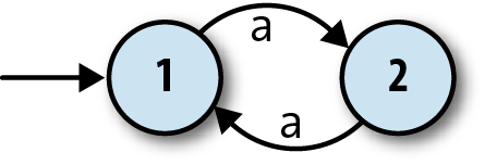
The two circles represent the automaton’s two states, 1 and 2, and
the arrow coming from nowhere shows that the automaton always starts in
state 1, its
start state
.
The arrows between states represent the rules of the
machine, which are:
When in state 1 and the character
ais read, move
into state 2.When in state 2 and the character
ais read, move
into state 1.
This is enough information for us to investigate how the machine
processes a stream of inputs:
The machine starts in state 1.
The machine only has rules for reading the character
afrom its input stream, so that’s the
only thing that can happen. When it reads ana, it moves from state 1 into state
2.When the machine reads another
a, it moves back into state 1.
Once it gets back to state 1, it’ll start repeating itself, so that’s the extent of this
particular machine’s behavior. Information about the current state is assumed to be internal
to the automaton—it operates as a “black box” that doesn’t reveal its inner workings—so the
boringness of this behavior is compounded by the uselessness of it not causing any kind of
observable output. Nobody in the outside world can see that anything is happening while the
machine is bouncing between states 1 and 2, so in this case, we might as well have a single
state and not bother with any internal structure at all.
To address this
problem, finite automata also have a rudimentary way of producing output. This
is nothing as sophisticated as the output capabilities of real computers; we just mark some
of the states as being special, and say that the machine’s single-bit output is the
information about whether it’s currently in a special state or not. For this machine, let’s
make state 2 a special state and show it on the diagram with a double circle:
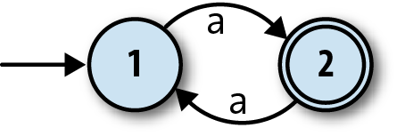
These special states are usually called
accept states
, which suggests the idea of a machine
accepting
or
rejecting
certain sequences of
inputs. If this automaton starts in state 1 and reads a singlea, it will be left in state 2, which is an accept state, so we can say that the
machine accepts the string'a'. On the other hand, if it
first reads anaand then anothera, it’ll end up back in state 1, which isn’t an accept state, so
the machine rejects the string'aa'. In fact, it’s easy
to see that this machine accepts any string ofas whose
length is an odd number:'a','aaa','aaaaa'are all accepted, while'aa','aaaa', and''(the empty string) are rejected.
Now we have something slightly more useful: a machine that can
read a sequence of characters and provide a yes/no output to indicate
whether that sequence has been accepted. It’s reasonable to say that
this DFA is performing a computation, because we can ask it a
question—“is the length of this string an odd number?”—and get a
meaningful reply back. This is arguably enough to call it a simple
computer, and we can see how its features stack up against a real
computer:
| | Real computer | Finite automaton |
| Permanent storage | Hard drive or SSD | None |
| Temporary storage | RAM | Current state |
| Input | Keyboard, mouse, network, etc. | Character stream |
| Output | Display device, speakers, network, etc. | Whether current state is an accept state (yes/no) |
| Processor | CPU core(s) that can execute any program | Hardcoded rules for changing state in response to input |
Of course, this specific automaton doesn’t do anything
sophisticated or useful, but we can build more complex automata that
have more states and can read more than one character. Here’s one with
three states and the ability to read the inputsaandb:

This machine accepts strings like'ab','baba', and'aaaab', and
rejects strings like'a','baa', and'bbbba'. A bit of experimentation
shows that it will only accept strings that contain the sequence'ab', which still isn’t hugely useful but at least demonstrates a degree of
subtlety. We’ll see more practical applications later in the
chapter.
Significantly, this
kind of automaton is
deterministic
:
whatever state it’s currently in, and whichever character it reads, it’s
always absolutely certain which state it will end up in. This certainty
is guaranteed as long as we respect two constraints:
No contradictions: there are no states where the machine’s
next move is ambiguous because of conflicting rules. (This implies
that no state may have more than one rule for the same input
character.)No omissions: there are no states where the machine’s next
move is unknown because of a missing rule. (This implies that every
state must have at least one rule for each possible input
character.)
Taken together, these constraints mean that the machine must have
exactly one rule for each combination of state and input. The technical
name for a machine that obeys the determinism constraints is a
deterministic finite automaton
(DFA).
Deterministic
finite automata are intended as abstract models of computation. We’ve drawn
diagrams of a couple of example machines and thought about their behavior, but these
machines don’t physically exist, so we can’t literally feed them input and see how they
behave. Fortunately DFAs are so simple that we can easily build a
simulation
of one in Ruby and interact with it directly.
Let’s begin building that simulation by implementing a collection
of
rules, which we’ll call a
rulebook
:
classFARule<Struct.new(:state,:character,:next_state)defapplies_to?(state,character)self.state==state&&self.character==characterenddeffollownext_stateenddefinspect"##{state.inspect}--#{character}-->#{next_state.inspect}>"endendclassDFARulebook<Struct.new(:rules)defnext_state(state,character)rule_for(state,character).followenddefrule_for(state,character)rules.detect{|rule|rule.applies_to?(state,character)}endend
This code establishes a simple API for rules: each rule has an#applies_to?method, which returnstrueorfalseto indicate whether that rule applies in
a particular situation, and a#followmethod that returns information about how the machine should change when
a rule is followed.
[
20
]DFARulebook#next_stateuses these methods to l
ocate the correct rule and discover what the next state of
the DFA should be.
By usingEnumerable#detect,
the implementation ofDFARulebook#next_stateassumes that there
will always be exactly one rule that applies to the given state and
character. If there’s more than one applicable rule, only the first
will have any effect and the others will be ignored; if there are
none, the#detectcall will returnniland the simulation will crash
when it tries to callnil.follow.
This is why the class is calledDFARulebookrather than justFARulebook: it only works properly if the
determinism constraints are respected.
A rulebook lets us wrap up many rules into a single object and ask
it questions about which state comes next:
>>rulebook=DFARulebook.new([FARule.new(1,'a',2),FARule.new(1,'b',1),FARule.new(2,'a',2),FARule.new(2,'b',3),FARule.new(3,'a',3),FARule.new(3,'b',3)])=> #>>rulebook.next_state(1,'a')=> 2>>rulebook.next_state(1,'b')=> 1>>rulebook.next_state(2,'b')=> 3
We had a choice here about how to represent the states of our automaton as Ruby
values. All that matters is the ability to tell the states apart: our implementation ofDFARulebook#next_stateneeds to be able to compare
two states to decide whether they’re the same, but otherwise, it doesn’t care whether
those objects are numbers, symbols, strings, hashes, or faceless instances of theObjectclass.
In this case, it’s clearest to use plain old Ruby numbers—they match up nicely with
the numbered states on the diagrams—so we’ll do that for now.
Once we have a rulebook, we can use it to build aDFAobject that keeps track of its current
state and can report whether it’s currently in an accept state or
not:
classDFA<Struct.new(:current_state,:accept_states,:rulebook)defaccepting?accept_states.include?(current_state)endend
>>DFA.new(1,[1,3],rulebook).accepting?=> true>>DFA.new(1,[3],rulebook).accepting?=> false
We can now write a method to read a character of input, consult
the rulebook, and change state accordingly:
classDFAdefread_character(character)self.current_state=rulebook.next_state(current_state,character)endend
This lets us feed characters to the DFA and watch its output
change:
>>dfa=DFA.new(1,[3],rulebook);dfa.accepting?=> false>>dfa.read_character('b');dfa.accepting?=> false>>3.timesdodfa.read_character('a')end;dfa.accepting?=> false>>dfa.read_character('b');dfa.accepting?=> true
Feeding the DFA one character at a time is a little unwieldy, so
let’s add a convenience method for reading an entire string of
input:
classDFAdefread_string(string)string.chars.eachdo|character|read_character(character)endendend
Now we can provide the DFA a whole string of input instead of
having to pass its characters individually:
>>dfa=DFA.new(1,[3],rulebook);dfa.accepting?=> false>>dfa.read_string('baaab');dfa.accepting?=> true
Once a DFA object has been fed some input, it’s probably not in its start state anymore,
so we can’t reliably reuse it to check a completely new sequence of inputs. That means we
have to recreate it from scratch—using the same start state, accept states, and rulebook as
before—every time we want to see whether it will accept a new string. We can avoid doing
this manually by wrapping up its constructor’s arguments in an object that represents the
design
of a particular DFA and relying on that object to
automatically build one-off instances of that DFA whenever we want to check for acceptance
of a string:
classDFADesign<Struct.new(:start_state,:accept_states,:rulebook)defto_dfaDFA.new(start_state,accept_states,rulebook)enddefaccepts?(string)to_dfa.tap{|dfa|dfa.read_string(string)}.accepting?endend
The#tapmethod evaluates a
block and then returns the object it was called on.
DFADesign#accepts?uses theDFADesign#to_dfamethod to create a
new instance ofDFAand then calls#read_string?to put it
into an accepting or rejecting state:
>>dfa_design=DFADesign.new(1,[3],rulebook)=> #>>dfa_design.accepts?('a')=> false>>dfa_design.accepts?('baa')=> false>>dfa_design.accepts?('baba')=> true