Understanding Computation (3 page)

Structis a special
Ruby class whose job is to generate other classes. A class
generated byStructcontains getter
and setter methods for each of the attribute names passed intoStruct.new. The conventional way to use aStruct-generated class is to subclass
it; the subclass can be given a name, and it provides a convenient place
to define any additional methods. For example, to make a class calledPointwith attributes calledxandy, we
can write:
classPoint<Struct.new(:x,:y)def+(other_point)Point.new(x+other_point.x,y+other_point.y)enddefinspect"##{x},#{y})>"endend
Now we can create instances ofPoint, inspect them in IRB, and send them
messages:
>>a=Point.new(2,3)=> #>>b=Point.new(10,20)=> #>>a+b=> #
As well as whatever methods we define, aPointinstance responds to the messagesxandx=to get and set the value of itsxattribute, and similarly foryandy=:
>>a.x=> 2>>a.x=35=> 35>>a+b=> #
Classes generated byStruct.newhave other useful
functionality, like an implementation of the
equality method#==, which compares the
attributes of twoStructs to see if they’re equal:
>>Point.new(4,5)==Point.new(4,5)=> true>>Point.new(4,5)==Point.new(6,7)=> false
New methods
can be added to an existing class or module at any time.
This is a powerful feature, usually called
monkey
patching
, which lets us extend the behavior of existing
classes:
>>classPointdef-(other_point)Point.new(x-other_point.x,y-other_point.y)endend=> nil>>Point.new(10,15)-Point.new(1,1)=> #
We can even monkey patch Ruby’s built-in classes:
>>classStringdefshoutupcase+'!!!'endend=> nil>>'hello world'.shout=> "HELLO WORLD!!!"
Ruby supports a
special kind of variable, called a
constant
, which should not be reassigned once
it’s been created. (Ruby won’t prevent a constant from being reassigned,
but it will generate a warning so we know we’re doing something bad.)
Any variable whose name begins with a capital letter is a constant. New
constants can be defined at the top level or within a
class or module:
>>NUMBERS=[4,8,15,16,23,42]=> [4, 8, 15, 16, 23, 42]>>classGreetingsENGLISH='hello'FRENCH='bonjour'GERMAN='guten Tag'end=> "guten Tag">>NUMBERS.last=> 42>>Greetings::FRENCH=> "bonjour"
Class and module names always begin with a capital letter, so
class and module names are constants too.
When we’re
exploring an idea with IRB it can be useful to ask Ruby to
forget about a constant altogether, especially if that constant is the
name of a class or module that we want to redefine from scratch instead
of monkey patching its existing definition. A top-level constant can be
removed by sending theremove_constmessage
toObject, passing the constant’s
name as a symbol:
>>NUMBERS.last=> 42>>Object.send(:remove_const,:NUMBERS)=> [4, 8, 15, 16, 23, 42]>>NUMBERS.lastNameError: uninitialized constant NUMBERS>>Greetings::GERMAN=> "guten Tag">>Object.send(:remove_const,:Greetings)=> Greetings>>Greetings::GERMANNameError: uninitialized constant Greetings
We have to useObject.send(:remove_const,instead of just
:NAME)Object.remove_const(:NAME)
becauseremove_constis a
private
method
that ordinarily can only be called by sending a message from inside theObjectclass itself; usingObject.sendallows us to bypass this restriction temporarily.
[
1
]
This style comes from the Smalltalk programming language, which
had a direct influence on the design of Ruby.
What is
computation
? The word itself means different things to different people, but everyone can agree that when a computer reads a program, runs that program, reads some input, and eventually produces some output, then some kind of computation has definitely happened. That gives us a decent starting point: computation is a name for
what a computer does
.
To create an environment where this familiar sort of computation can occur, we need three basic ingredients:
A
machine
capable of performing the computationA
language
for writing instructions that the machine can
understandA
program
written in that language, describing the exact
computation that the machine should perform
So this part of the book is about machines, languages, and programs—what they are, how
they behave, how we can model and study them, and how we can exploit them to get useful work
done. By investigating these three ingredients, we can develop a better intuition for what
computation is and how it happens.
In
Chapter 2
, we’ll design and implement a toy programming
language by exploring several different ways to specify its meaning. Understanding the meaning
of a language is what allows us to take a lifeless piece of source code and animate it as a
dynamic, executing process; each specification technique gives us a particular strategy for
running a program, and we’ll end up with several different ways of implementing the same
language.
We’ll see that programming is the art of assembling a precisely defined structure that
can be dismantled, analyzed, and ultimately interpreted by a machine to create a
computation. And more important, we’ll discover that implementing programming languages is
easy and fun: although parsing, interpretation, and compilation can seem intimidating, they’re
actually quite simple and enjoyable to play around with.
Programs aren’t much use without machines to run them on, so in
Chapter 3
, we’ll design very simple machines capable of performing
basic, hardcoded tasks. From that humble foundation, we’ll work our way up to more
sophisticated machines in
Chapter 4
, and in
Chapter 5
, we’ll see how to design a general-purpose computing device
that can be controlled with software.
By the time we reach
Part II
, we’ll have seen the
full spectrum of computational power: some machines with very limited capabilities, others
that are more useful but still frustratingly constrained, and finally, the most powerful
machines that we know how to build.
Don’t think,
feel
! It is like a finger pointing
away to the moon. Don’t concentrate on the finger or you will miss all
that heavenly glory.
Bruce Lee
Programming languages,
and the programs we write in them, are fundamental to our work as software
engineers. We use them to clarify complex ideas to ourselves, communicate those ideas to each
other, and, most important, implement those ideas inside our computers. Just as human society
couldn’t operate without natural languages, so the global community of programmers relies on
programming languages to transmit and implement our ideas, with each successful program forming
part of a foundation upon which the next layer of ideas can be built.
Programmers tend to be practical, pragmatic creatures. We often learn
a new programming language by reading documentation, following tutorials,
studying existing programs, and tinkering with simple programs of our own,
without giving much thought to what those programs
mean
. Sometimes the learning process feels a lot like
trial and error: we try to understand a piece of a language by looking at
examples and documentation, then we try to write something in it, then
everything blows up and we have to go back and try again until we manage to
assemble something that mostly works. As computers and the systems they
support become increasingly complex, it’s tempting to think of programs as
opaque incantations that represent only themselves and work only by
chance.
But computer programming isn’t really about
programs
, it’s about
ideas
.
A program is a frozen representation of an idea, a snapshot of a structure that once
existed in a programmer’s imagination. Programs are only worth writing because they have
meaning
. So what connects code to its meaning, and how can we be more
concrete about the meaning of a program than saying “it just does whatever it does”? In this
chapter, we’re going to look at a few techniques for nailing down the meanings of computer
programs and see how to bring those dead snapshots to life.
In linguistics,
semantics
is the study of the connection between words and their
meanings: the word “dog” is an arrangement of shapes on a page, or a
sequence of vibrations in the air caused by someone’s vocal cords, which
are very different things from an actual dog or the idea of dogs in
general. Semantics is concerned with how these concrete signifiers relate
to their abstract meanings, as well as the fundamental nature of the
abstract meanings themselves.
In computer science, the field of
formal
semantics
is
concerned with finding ways of nailing down the elusive
meanings of programs and using them to discover or prove interesting
things about programming languages. Formal semantics has a wide spectrum
of uses, from concrete applications like specifying new languages and
devising compiler optimizations, to more abstract ones like constructing
mathematical proofs of the correctness of programs.
To completely specify a
programming language, we need to provide two things:
a
syntax
, which describes what programs look like, and a semantics,
[
2
]
which describes what programs mean.
Plenty of languages don’t have an official written specification,
just a working interpreter or compiler. Ruby itself falls into
this “specification by implementation” category: although
there are plenty of books and tutorials about how Ruby is supposed to
work, the ultimate source of all this information is
Matz’s Ruby Interpreter (MRI), the language’s reference
implementation. If any piece of Ruby documentation disagrees with the
actual behavior of MRI, it’s the documentation that’s wrong; third-party
Ruby implementations like JRuby, Rubinius, and MacRuby have to work hard
to imitate the exact behavior of MRI so that they can usefully claim to be
compatible with the Ruby language. Other languages like PHP and Perl 5
share this implementation-led approach to language definition.
Another way of describing a programming language is to write an
official prose specification, usually in English. C++, Java, and
ECMAScript (the standardized version of JavaScript) are examples of this
approach: the languages are standardized in implementation-agnostic
documents written by expert committees, and many compatible
implementations of those standards exist. Specifying a language with an
official document is more rigorous than relying on a reference
implementation—design decisions are more likely to be the result of
deliberate, rational choices, rather than accidental consequences of a
particular implementation—but the specifications are often quite difficult
to read, and it can be very hard to tell whether they contain any
contradictions, omissions, or ambiguities. In particular there’s no formal
way to reason about an English-language specification; we just have to
read it thoroughly, think about it a lot, and hope we’ve understood all
the
consequences.
A prose specification of Ruby 1.8.7 does exist, and has even been
accepted as an ISO standard (ISO/IEC 30170).
[
3
]
MRI is still regarded as the canonical
specification-by-implementation of the Ruby language, although the
mruby project
is an
attempt to build a lightweight, embeddable Ruby implementation that
explicitly aims for compliance with the ISO standard rather than MRI
compatibility.
A third alternative is to use the mathematical techniques of formal
semantics to precisely describe the meaning of a programming language. The
goal here is to be completely unambiguous, as well as to write the
specification in a form that’s suited to methodical analysis, or even
automated
analysis, so that it can be comprehensively
checked for consistency, contradiction, or oversight. We’ll look at these
formal approaches to semantic specification after we’ve seen how syntax is
handled.
A conventional
computer program is a long string of characters. Every
programming language comes with a collection of rules that describe what
kind of character strings may be considered valid programs in that
language; these rules specify the language’s
syntax
.
A language’s syntax rules allow us to distinguish potentially valid programs likey = x + 1from nonsensical ones like>/;x:1@4. They also provide useful information about how to read ambiguous
programs: rules about operator precedence, for example, can automatically determine that1 + 2 * 3should be treated as though it had been written
as1 + (2 * 3), not as(1 + 2) *.
3
The intended use of a computer program is, of course, to be read by
a computer, and reading programs requires a
parser
: a program that can read a
character string representing a program, check it against the syntax rules
to make sure it’s valid, and turn it into a structured representation of
that program suitable for further processing.
There are a variety of tools that can automatically turn a language’s syntax
rules into a parser. The details of how these rules are specified, and the
techniques for turning them into usable parsers, are not the focus of this chapter—see
Implementing Parsers
for a quick overview—but overall, a parser should read a
string likey = x + 1and turn it into
an
abstract syntax tree
(AST), a representation of the
source code that discards incidental detail like whitespace and focuses on the hierarchical
structure of the program.
In the end, syntax is only concerned with the surface appearance of
programs, not with their meanings. It’s possible for a program to be syntactically
valid but not mean anything useful; for example, it might be that the programy = x + 1doesn‘t make sense on its own because it doesn’t say
whatxis beforehand, and the programz = true + 1might turn out to be broken when we run it because
it’s trying to add a number to a Boolean value. (This depends, of course, on other properties
of whichever programming language we’re talking about.)
As we might expect, there is no “one true way” of explaining how the syntax of a
programming language corresponds to an underlying meaning. In fact there are several different
ways of talking concretely about what programs mean, all with different trade-offs between
formality, abstraction, expressiveness, and practical efficiency. In the next few sections,
we’ll look at the main formal approaches and see how they relate to each other.
The most
practical way to think about the meaning of a program is
what it does
—when we run the program, what do we
expect to happen? How do different constructs in the programming language
behave at run time, and what effect do they have when they’re plugged
together to make larger programs?
This is the basis of
operational semantics
, a way of capturing the
meaning of a programming language by defining rules for how its programs execute on some kind
of device. This device is often an
abstract machine
: an imaginary, idealized computer that is designed for
the specific purpose of explaining how the language’s
programs will execute. Different kinds of
programming language will usually require different designs of abstract machine in
order to neatly capture their runtime behavior.
By giving an operational semantics, we can be quite rigorous and precise about the purpose
of particular constructs in the language. Unlike a language specification written in English,
which might contain hidden ambiguities and leave important edge cases uncovered, a formal
operational specification will need to be explicit and unambiguous in order to convincingly
communicate the language’s behavior.
So, how can we
design an abstract machine and use it to specify the
operational semantics of a programming language? One way is to imagine a
machine that evaluates a program by operating on its syntax directly,
repeatedly
reducing
it in small steps, with each
step bringing the program closer to its final result, whatever that
turns out to mean.
These small-step
reductions are similar to the way we are taught in school to evaluate algebraic
expressions. For example, to evaluate (1 × 2) + (3 × 4), we know we should:
Perform the left-hand multiplication (1 × 2 becomes 2) and reduce the expression to
2 + (3 × 4)Perform the right-hand multiplication (3 × 4 becomes 12) and reduce the expression
to 2 + 12Perform the addition (2 + 12 becomes 14) and end up with 14
We can think of 14 as the result because it can’t be reduced any further by this
process—we recognize 14 as a special kind of algebraic expression
, a
value
, which has its own meaning and doesn’t require
any more work on our part.
This informal process can be turned into an operational semantics
by writing down formal rules about how to proceed with each small
reduction step. These rules themselves need to be written in some
language (the
metalanguage
), which
is usually mathematical notation.
In this chapter, we’re going to explore the semantics of a toy programming
language—let’s call it
Simple
.
[
4
]
The mathematical description of
Simple
’s small-step semantics
looks like this:
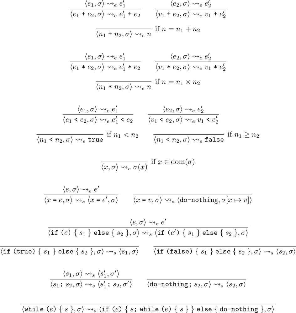
Mathematically speaking, this is a
set of
inference rules
that defines
a
reduction relation
on
Simple
’s abstract syntax trees. Practically
speaking, it’s a bunch of weird symbols that don’t say anything
intelligible about the meaning of computer programs.
Instead of trying to understand this formal notation directly,
we’re going to investigate how to write the same inference rules in
Ruby. Using Ruby as the metalanguage is easier for a programmer to
understand, and it gives us the added advantage of being able to execute
the rules to see how they work.
We are
not
trying to describe the semantics
of
Simple
by giving a “specification
by implementation.” Our main reason for describing the small-step
semantics in Ruby instead of mathematical notation is to make the
description easier for a human reader to digest. Ending up with an
executable implementation of the language is just a nice bonus.
The big disadvantage of using Ruby is that it explains a simple
language by using a more complicated one, which perhaps defeats the
philosophical purpose. We should remember that the mathematical rules
are the authoritative description of the semantics, and that we’re
just using Ruby to develop an understanding of what those rules
mean.
We’ll start by
looking
at the semantics of
Simple
expressions. The rules will operate
on the abstract syntax of these expressions, so we need to be able to
represent
Simple
expressions as Ruby
objects. One way of doing this is to define a Ruby class for each
distinct kind of element from
Simple
’s syntax—numbers, addition,
multiplication, and so on—and then represent each expression as a tree
of instances of these classes.
For example, here are the definitions ofNumber,Add, andMultiplyclasses:
classNumber<Struct.new(:value)endclassAdd<Struct.new(:left,:right)endclassMultiply<Struct.new(:left,:right)end
We can
instantiate these classes to
build abstract syntax trees by hand:
>>Add.new(Multiply.new(Number.new(1),Number.new(2)),Multiply.new(Number.new(3),Number.new(4)))=> #left=#left=#, right=#>,right=#left=#, right=#>>
Eventually, of course, we want these trees to be built
automatically by a parser. We’ll see how to do that in
Implementing Parsers
.
TheNumber,Add, andMultiplyclasses inheritStruct’s generic
definition of#inspect, so the
string representations of their instances in the IRB console contain a
lot of unimportant detail. To make the content of an abstract syntax
tree easier to see in IRB, we’ll override#inspecton each class
[
5
]
so that it returns a custom string
representation:
classNumberdefto_svalue.to_senddefinspect"«#{self}»"endendclassAdddefto_s"#{left}+#{right}"enddefinspect"«#{self}»"endendclassMultiplydefto_s"#{left}*#{right}"enddefinspect"«#{self}»"endend
Now each abstract syntax tree will be shown in IRB as a short
string of
Simple
source code,
surrounded by
«guillemets» to distinguish it from a normal Ruby
value:
>>Add.new(Multiply.new(Number.new(1),Number.new(2)),Multiply.new(Number.new(3),Number.new(4)))=> «1 * 2 + 3 * 4»>>Number.new(5)=> «5»
Our rudimentary#to_simplementations don’t take
operator precedence into account, so sometimes their output is incorrect with respect to
conventional precedence rules (e.g.,*usually binds
more tightly than+). Take this abstract syntax tree,
for example:
>>Multiply.new(Number.new(1),Multiply.new(Add.new(Number.new(2),Number.new(3)),Number.new(4)))=> «1 * 2 + 3 * 4»
This tree represents «1 * (2 + 3) *», which is a different expression (with a different
4
meaning) than «1 * 2 + 3 * 4»,
but its string representation doesn’t reflect that.
This problem is serious but tangential to our discussion of semantics. To keep
things simple, we’ll temporarily ignore it and just avoid creating expressions that have
an incorrect string representation. We’ll implement a proper solution for another
language in
Syntax
.
Now we can begin to implement a small-step
operational semantics by defining methods that perform
reductions on our abstract syntax trees—that is, code that can take an
abstract syntax tree as input and produce a slightly reduced tree as
output.
Before we can implement reduction itself, we need to be able to
distinguish expressions that can be reduced from those that can’t.AddandMultiplyexpressions are always
reducible—each of them represents an operation, and can be turned into
a result by performing the calculation corresponding to that
operation—but aNumberexpression
always represents a value, which can’t be reduced to anything
else.
In principle, we could tell these two kinds of expression apart with a single#reducible?predicate that returnstrueorfalsedepending on the class of
its argument:
defreducible?(expression)caseexpressionwhenNumberfalsewhenAdd,Multiplytrueendend
In Rubycasestatements,
the control expression is matched against the cases by calling each
case value’s#===method with the
control expression’s value as an argument. The implementation of#===for class objects checks to
see whether its argument is an instance of that class or one of its
subclasses, so we can use thecasesyntax to match anobjectwhenclassname
object against a class.
However, it’s generally
considered bad form to write code like this in an
object-oriented language;
[
6
]
when the behavior of some operation depends upon the
class of its argument, the typical approach is to implement each
per-class behavior as an instance method for that class, and let the
language implicitly handle the job of deciding which of those methods
to call instead of using an explicitcasestatement.
So instead, let’s implement separate#reducible?methods forNumber,Add, andMultiply:
classNumberdefreducible?falseendendclassAdddefreducible?trueendendclassMultiplydefreducible?trueendend
This gives us the behavior we want:
>>Number.new(1).reducible?=> false>>Add.new(Number.new(1),Number.new(2)).reducible?=> true
We can now implement reduction for these expressions; as above, we’ll do this by
defining a#reducemethod forAddandMultiply. There’s no need to
defineNumber#reduce, since numbers can’t be reduced,
so we’ll just need to be careful not to call#reduceon
an expression unless we know it’s reducible.
So what are the rules for reducing an addition expression? If the left and right
arguments are already numbers, then we can just add them together, but what if one or both
of the arguments needs reducing? Since we’re thinking about small steps, we need to decide
which argument gets reduced first if they are both eligible for reduction.
[
7
]
A common strategy is to reduce the arguments in left-to-right order, in which
case the rules will be:
If the addition’s left argument can be reduced, reduce the left argument.
If the addition’s left argument can’t be reduced but its right argument can,
reduce the right argument.If neither argument can be reduced, they should both be numbers, so add them
together.
The structure of these rules is characteristic of small-step operational semantics.
Each rule provides a pattern for the kind of expression to which it applies—an addition
with a reducible left argument, with a reducible right argument, and with two irreducible
arguments respectively—and a description of how to build a new, reduced expression when
that pattern matches. By choosing these particular rules, we’re specifying that a
Simple
addition expression uses left-to-right evaluation to
reduce its arguments, as well as deciding how those arguments should be combined once
they’ve been individually reduced.
We can translate these rules directly into an implementation ofAdd#reduce, and almost the same
code will work forMultiply#reduce(remembering to multiply the arguments instead of adding them):
classAdddefreduceifleft.reducible?Add.new(left.reduce,right)elsifright.reducible?Add.new(left,right.reduce)elseNumber.new(left.value+right.value)endendendclassMultiplydefreduceifleft.reducible?Multiply.new(left.reduce,right)elsifright.reducible?Multiply.new(left,right.reduce)elseNumber.new(left.value*right.value)endendend