101 Excel 2013 Tips, Tricks and Timesavers (2 page)
Read 101 Excel 2013 Tips, Tricks and Timesavers Online
Authors: John Walkenbach

Part I: Workbooks and Files
In this part, you’ll find tips and tricks covering some of the basics of Excel, including Protected View and AutoRecover, as well as working with the Quick Access toolbar and charging Excel’s color scheme.
Tips and Where to Find Them
Tip 1:
Changing the Look of Excel
Tip 2:
Customizing the Quick Access Toolbar
Tip 4:
Understanding Protected View
Tip 5:
Understanding AutoRecover
Tip 6:
Using a Workbook in a Browser
Tip 7:
Saving to a Read-Only Format
Tip 8:
Generating a List of Filenames
Tip 9:
Generating a List of Sheet Names
Tip 10:
Using Document Themes 32
Tip 1: Changing the Look of Excel
With Excel 2013, what you see isn’t necessarily what you have to live with. This tip describes several ways to change the look of Excel. Some changes affect only the appearance. Other options allow you to hide various parts of Excel to make more room for displaying your data — or maybe because you prefer a less-cluttered look.
Cosmetic changes
When the preview version of Microsoft Office 2013 became available, there was a minor uproar about its appearance. Compared to previous versions, the applications looked “flat” and many complained about the overall white color.
When the final version was released, Microsoft added two alternative Office themes: light gray and dark gray. To switch to a different theme, choose File⇒Options to display the Excel Options dialog box. Click the General tab and use the Office Theme drop-down list (see Figure 1-1). The theme choice affects the appearance of the title bar, row and column borders, task panes, the taskbar, and a few other items. The theme you choose applies to all other Office 2013 applications.
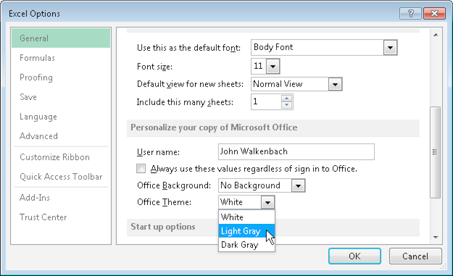
Figure 1-1:
Selecting a different Office theme.
Figure 1-1 shows another option: Office Background. Use this drop-down list to select a background image that appears in the Excel title bar. Fortunately, one of the options is No Background.
Hiding the Ribbon
To hide the Ribbon, click the Ribbon Display Options drop-down menu in the Excel title bar. You’ll see the choices shown in Figure 1-2.
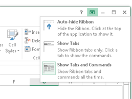
Figure 1-2:
Choosing how the Ribbon works.
Using options on the View tab
The View tab, shown in Figure 1-3, has three groups of commands that determine what you see onscreen.
→
Workbook Views group:
These options control the overall view. Most of the time, you’ll use Normal view. Page Layout view is useful if you require precise control over how the pages are laid out. Page Break Preview also shows page breaks, but the display isn’t nearly as nice. The status bar has icons for each of these views. Custom Views enable you to create named views of worksheet settings (for example, a view in which certain columns are hidden).
→
Show group:
The four checkboxes in this group control the visibility of the Ruler (relevant only in Page Layout view), the Formula bar, worksheet gridlines, and row and column headings.
→
Zoom group:
These commands enable you to zoom the worksheet in or out. Another way to zoom is to use the Zoom slider on the status bar.
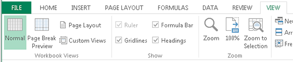
Figure 1-3:
Controls on the View tab.
Hiding other elements
To hide other elements, you must make a trip to the Advanced tab of the Excel Options dialog box (choose File⇒Options). Figure 1-4 shows workbook display options and worksheet display options. These options are self-explanatory.
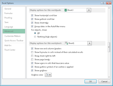
Figure 1-4:
Display options on the Advanced tab of the Excel Options dialog box.
Hiding the status bar
You can also hide the status bar, at the bottom of the Excel window. Doing so, however, requires VBA code.
1.
Press Alt+F11 to display the Visual Basic Editor.
2.
Press Ctrl+G to display the Immediate window.
3.
Type this statement and press Enter:
Application.DisplayStatusBar = False
The status bar will be removed from all open workbook windows. To redisplay the status bar, repeat those instructions, but specify True in the statement.
Tip 2: Customizing the Quick Access Toolbar
If you find that you continually need to switch Ribbon tabs because a frequently used command never seems to be on the Ribbon that’s displayed, this tip is for you. The Quick Access toolbar is always visible, regardless of which Ribbon tab is selected. After you customize the Quick Access toolbar, your frequently used commands will always be one click away.
 The only situation in which the Quick Access toolbar is not visible is when the title bar is hidden (by choosing Auto-Hide the Ribbon from the Ribbon Display Options drop-down list in the title bar).
About the Quick Access toolbar
By default, the Quick Access toolbar is located on the left side of the Excel title bar, and it includes three tools:
→
Save:
Saves the active workbook.
→
Undo:
Reverses the effect of the last action.
→
Redo:
Reverses the effect of the last undo.
Commands on the Quick Access toolbar always appear as small icons, with no text. When you hover your mouse pointer over an icon, you see the name of the command and a brief description.
As far as I can tell, the number of icons that you can add to your Quick Access toolbar is limitless. But regardless of the number of icons, the Quick Access toolbar always displays a single line of icons. If the number of icons exceeds the Excel window width, it displays an additional icon at the end: More Controls. Click the More Controls icon, and the hidden Quick Access toolbar icons appear in a pop-up window.
Adding new commands to the Quick Access toolbar
You can add a new command to the Quick Access toolbar in three ways:
→ Click the Quick Access toolbar drop-down control, which displays a down-pointing arrow and is located on the right side of the Quick Access toolbar (see Figure 2-1). The list contains several commonly used commands. Select a command from the list, and Excel adds it to your Quick Access toolbar.
→ Right-click any control on the Ribbon and choose Add to Quick Access Toolbar. The control is added to your Quick Access toolbar, positioned after the last control.
→ Use the Quick Access Toolbar tab of the Excel Options dialog box. A quick way to access this dialog box is to right-click any Quick Access toolbar or Ribbon control and choose Customize Quick Access Toolbar.
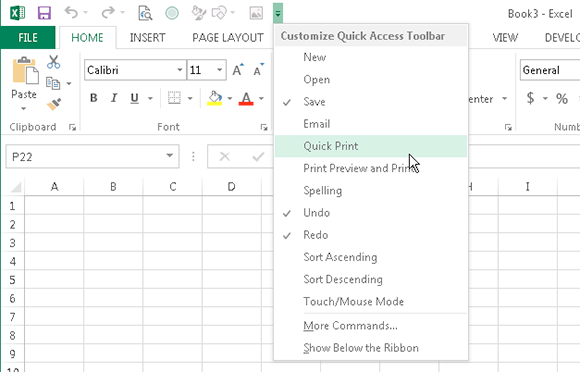
Figure 2-1:
The Quick Access toolbar drop-down menu is one way to add a new command to the Quick Access toolbar.
Figure 2-2 shows the Quick Access Toolbar tab of the Excel Options dialog box. The left side of the dialog box displays a list of Excel commands, and the right side shows the commands that are now on the Quick Access toolbar. Above the command list on the left is a drop-down control that lets you filter the list. Select an item from the drop-down list, and the list displays only the commands for that item.
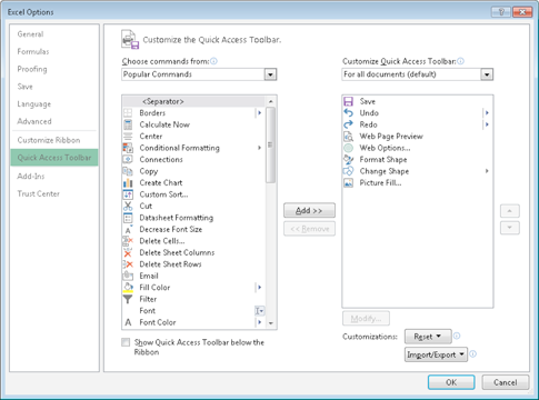
Figure 2-2:
Use the Quick Access Toolbar tab in the Excel Options dialog box to customize the Quick Access toolbar.
Some of the items in the drop-down list are described here:
→
Popular Commands:
Displays commands that Excel users commonly use.
→
Commands Not in the Ribbon:
Displays a list of commands that you cannot access from the Ribbon.
→
All Commands:
Displays a complete list of Excel commands.
→
Macros:
Displays a list of all available macros.
→
File Tab:
Displays the commands available in the back stage window.
→
Home Tab:
Displays all commands that are available when the Home tab is active.