Life's Ratchet: How Molecular Machines Extract Order from Chaos (21 page)
Read Life's Ratchet: How Molecular Machines Extract Order from Chaos Online
Authors: Peter M. Hoffmann

Imagine a map representing the energy of any possible shape of a protein. The coordinates of the map (north, west, south, and east) represent
the angles of the links, and the topographic height, at each coordinate, represents the corresponding energy. This creates what physicists call the energy landscape of the protein.
Figure 4.4
shows possible shapes of a short protein chain with the associated energy shown as the height on the landscape. The protein shown in this schematic has just four links, while real proteins consist of thousands of amino acid links, making the energy landscape fantastically complicated. The different links of the protein are randomly pushed around by the molecular storm, causing the protein to continuously change shape. This ongoing change in shape is represented by the white path across the landscape. Each location along the path corresponds to a specific shape of the protein (some examples are shown in the figure).
Sometimes the molecular storm pushes the protein into an uncomfortable, high-energy shape (a hill in the landscape); quickly, the protein relaxes down the hill to a more comfortable configuration. When the protein shape approaches the optimal shape, its energy reduces and it falls into an energy funnel in the landscape. Further reduction in energy draws the protein to the bottom of the funnel, where it assumes its lowest-energy configuration and optimal final shape.
As the molecular storm pushes the protein around, the succession of different protein shapes can be represented as a meandering path across the (abstract) energy landscape (the white path in
Figure 4.4
). Physicists talk about a diffusion across the energy landscape (diffusion here means random motion). Without the molecular storm, the molecule would be stuck in a fixed shape and would never find the optimal shape that minimizes its free energy. The diffusion across the energy landscape is a search that eventually leads the protein molecule to its optimal, lowest-energy shape. This optimal shape of the protein determines the function of the protein. Without its three-dimensional shape, a protein is nothing. The particular sequence of amino acids making up the protein has meaning only as far as it determines the protein’s 3-D shape.
For some proteins, the search for the optimal shape would simply take too long. For such proteins, life invented smaller proteins that chaperone, or guide, the larger molecule toward its proper shape. These
chaperonin molecules
serve as local molds that preshape parts of a protein and help it find its way along the energy landscape more quickly.
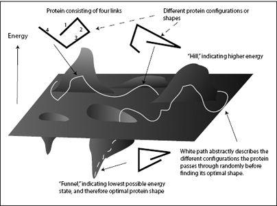
FIGURE 4.4.
The energy landscape of folding a protein.
Protein folding is possibly the best example of how physical laws, randomness, and information—provided by evolution—work together to create life’s complexities. The amino acid sequence of a protein is determined by the cell’s DNA, according to the genetic code. This information evolved over billions of years. But the information in our DNA
only
encodes the amino acid sequence; it does not encode the final 3-D shape of the protein. The 3-D shape is a result of the energy landscape, which is determined by physical forces (hydrophobic forces, electrostatic forces, bending energies, etc.) acting on the particular sequence of amino acids. This shape also depends on external conditions (pH, temperature, ion concentration). Thus a large part of the necessary information to form a protein is not contained in DNA, but rather in the physical laws governing charges, thermodynamics, and mechanics. And finally,
randomness
is needed to allow the amino acid chain to search the space of possible shapes and to find its optimal shape.
Erwin Schrödinger wondered how life’s molecules, especially DNA, could remain stable under the onslaught of the molecular storm. He postulated that stability is provided by strong chemical bonds. He was partly right—there are strong chemical bonds along the backbone of both DNA and proteins—but he missed the most interesting point: The functional structure of the large molecules in cells is not held together by a few strong bonds, but by many relatively weak ones, especially hydrogen bonds, but also hydrophobic interactions and so-called disulfide bridges (bonds between sulfur atoms attached to sulfur-containing amino acids in a protein). If the unique coil shape of a protein and the double helix of a DNA strand are held together by weak bonds, why are these shapes so stable?
If all bonds in the molecules of living organisms are too strong, there can be no motion or change. If they’re too weak, there can be no stability. The key is to find a middle ground between stability and flexibility. If things are too stable, they cannot function—imagine a car with lead wheels. If they are too flexible and fragile, they cannot function either. The solution that life has found is to capitalize on the cooperativity of many bonds. As we saw earlier, many weak bonds cooperating make a molecule very strong, while individually, the bonds can easily be broken, allowing for rearrangement when needed.
How can bonds be cooperative? In the aforementioned micelle, molecules act cooperatively to form a larger structure. If we replace
molecule
with
bond
, we have a similar situation. Once a DNA molecule is formed, the two strands of the DNA are held together by numerous hydrogen bonds. A single hydrogen bond can easily break at room temperature. The average lifetime of a hydrogen bond in water at room temperature is in the picosecond range (that is, a thousandth of a billionth of a second). However, if we have many hydrogen bonds working together, the spontaneous separation of two DNA strands would require a simultaneous,
cooperative
breaking of a large number of bonds—and this will not happen spontaneously. Single bonds may temporarily break in a DNA molecule, but they will quickly reform—forced back together by the presence of
neighboring hydrogen bonds, which keep the DNA molecule in shape. In living cells, DNA retains its double-helix structure when the molecule is not in use. However, when the information contained in DNA needs to be read out, the double helix must be opened up. This is achieved by specialized proteins, which locally lower the barrier to undo a number of hydrogen bonds and, like a zipper, unzip the DNA where needed and then close it back up (see
Chapter 7
for more on this).
Stability in DNA is also actively achieved by repair enzymes. If for some reason a part of the DNA molecule becomes corrupted, the repair enzymes will fix the mistake, using an adjacent section of the molecule that is undamaged as a chemical template to repair the corrupted part. The stability of DNA is therefore the result of bond cooperativity, complementarity of the two strands, and active repair by the cell’s machinery.
The situation is similar for proteins. A protein’s shape is held together by hydrophobic, hydrogen, and disulfide bonds, again cooperatively stabilizing the shape of the protein. The protein’s particular amino acid sequence is chosen by evolution such that a protein is just flexible enough to do its job (we will find out in the next chapters what kind of jobs they do) while keeping its overall shape. If a protein does get out of shape, the cell quickly discards it and recycles it back into its components.
Cooperativity is almost inevitable when you have many entities interacting with each other. I found this out in my own research when my students and I looked at simple liquids—water or oil—squeezed down to a few nanometers. While solids, in the form of crystals, have long-range order (atoms are arranged in an orderly pattern over large distances throughout the crystal), liquids have short-range order: If you were sitting on a water molecule in a pool of liquid water, you would see neighboring molecules at an average distance of 0.25 nanometer (nm). These neighbors would move around, but on average, there would be a cloud of water molecules surrounding you at this distance. Beyond this distance, the next-nearest neighbors would feel the presence of your neighbors, and you would see an excess of molecules at an average distance of 2 × 0.25 nm =
0.5 nm. However, because of the incessant motion of all molecules, this excess of molecules at 0.5 nm would be a little bit more smeared-out than the excess of molecules at 0.25 nm. Going even further, there would be an even more smeared-out excess at 0.75 nm and so on, until at a distance of five to six molecular diameters, thermal motion would have smeared out any semblance of order, and water molecules could be found with equal probability at just about any distance.
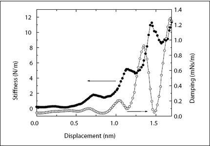
In my laboratory, we are using a different method to probe the short-range order of liquids. When liquids encounter a solid surface, they arrange themselves into molecular layers. The first layer, closest to the surface, is well defined. There is a high probability that we find water molecules at 0.25 nm from the surface. The second layer is a little bit more diffuse, and as we move away from the surface, the layers become more and more smeared-out, until order vanishes altogether after about five or six layers, as discussed above. This layering can be measured by an AFM. In our lab, we immerse an AFM cantilever and probe tip into water and then slowly move the tip toward the surface. To measure the response of the intervening water, we oscillate the tip at an amplitude (size of oscillating motion) of less than 0.1 nm—the diameter of a single hydrogen atom! Monitoring the amplitude, which changes slightly as we push through the water layers, we measure the “springiness” of the water layers (or “stiffness,” as we call it), that is, the capacity of water to push back at the tip if we push the tip against it. The stiffness fluctuates up and down with a period of 0.25 nm—the size of the water molecules—illustrating the molecular graininess of the liquid. An example of such a measurement is shown in
Figure 4.5
.
In 2006, my post-doc Shiva Patil and my student George Matei were performing such measurements on a silicone oil, octamethyl-cyclo-tetrasiloxane. OMCTS has large molecules (if you are a nanoscientist), with diameters of 1 nm. Together with the stiffness, we also measured the damping of the liquid layers. While the stiffness tells us how much the liquid layers spring back into their original shape (i.e., how much energy they store), the damping tells us how much energy is lost as we push on the layers. The damping also fluctuated with the spacing between the tip and the surface, with the same period as the stiffness. Looking at the data, Shiva noticed something peculiar: The damping fluctuation wasn’t always in line with the fluctuations of the stiffness. Sometimes the peaks in the damping lined up with the peaks in the stiffness, but sometimes they were switched—peaks in damping coincided with valleys in the stiffness. What was the difference between the measurements? We looked at everything—ion concentration, liquid purity, problems with the instrument. After two weeks, Shiva found that the difference between the measurements was in the speed at which the tip approached the surface. Yet, we were moving the tip so slowly in our measurements—the fastest speed we used was 1.2 nm per second—that it shouldn’t have mattered. At this extremely slow speed, it would take almost a second to push the tip through one layer of molecules. For liquid molecules at room temperature, a second might as well be an eternity. Thermal motion is much, much faster than this. Yet, we found that something quite dramatic happened when we went from a speed of 0.4 nm per second to 0.6 nm per second and beyond. At the slower speeds, damping and stiffness fluctuated together. This meant that the liquid behaved like a liquid—it just got thicker and thinner as we pushed the tip through. At faster speeds, the liquid assumed a new state; it became springy with very little energy loss. Usually, only solids could do this. Since then, we have found the same effect in liquid water, although here we have had to squeeze a little bit faster to make it happen. Water is still liquid at 0.8 nm per second and starts behaving like a solid beyond that speed. The transition between the two states of the liquid is extremely sharp: Below a critical speed, it always behaves like a liquid, and within a very small range of speeds, it completely switches to a solid-like response.