X and the City: Modeling Aspects of Urban Life (40 page)
Read X and the City: Modeling Aspects of Urban Life Online
Authors: John A. Adam

If we let
b
= (1 +
α
)
a
, this can be rearranged to give

The parameter
α
is a measure of how “rectangular” the town center is; the smaller the value of
α
the closer the center is to being square. Furthermore, since we wish to write and
and
A
=
ab
= (1 +
α
)
a
2
, it follows that

This can be simplified still further by noting that, since
a
=
m
Δ and
b
=
n
Δ,

Substituting for
n
we find that, after a little rearrangement,

Figure 14.2
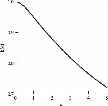
shows excellent agreement for bounds on
k
(
α
) when compared with the range quoted by Smeed. In passing, it is worthwhile to note that the topics discussed here are related to the probabilistic one of determining the average distance between two random points in a circle. A simple derivation of one such result can be found in
Appendix 7
. There has been much in the mathematical literature devoted to this problem, and it has been adapted by several theoretical urban planning groups to model optimal traffic routes between centers of interest.

Figure 14.2. Proportionality parameter
k
(see equation (14.5)) as a function of
α
(
m
= 10 here).
X
=
T
i
: Question:
What difference does a beltway make?
A beltway (or ring road in the UK) is a highway that encircles an urban area so that traffic does not necessarily have to pass through the center. A driver wishing to get to the other side of the city without going through the center might be well advised to use this alternative route. However, I’ve heard it said regarding the M25 motorway (a beltway around outer London) that it can be the largest parking lot in the world at times! Nevertheless, in my (somewhat limited) experience, a combination of variable speed limits and traffic cameras usually keeps the traffic flowing quite efficiently via a feedback mechanism between the two.
As always in our simple models, circular cities will be considered to be radially symmetric; that is, properties vary only with distance
r
. The city is of radius
r
0
and
v
(
r
) is the speed of traffic (in mph) at a distance
r
from the city center, 0 ≤
r
≤
r
0
.
V
0
is the speed of traffic around the (outer) beltway from any starting point
A
on the perimeter. For simplicity we will assume that
V
0
is constant and that
v
(
r
) is a linearly increasing function; as we will see, even these simplistic assumptions are sufficient to provide some insight into the potential advantages of a beltway. Thus
v
(
r
) =
ar
+
b
,
a
≥ 0,
b
≥ 0. A driver wishes to travel from point
A
to point
P
(
r
0
,
θ
), (see
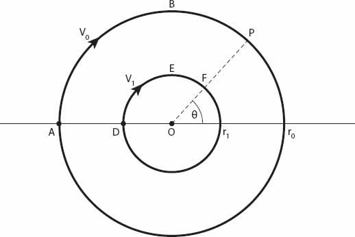
Figure 14.3
) both situated on the perimeter road. We shall suppose that there is also a circular “inner city” beltway a distance
r
1
<
r
0
from the center
O
, along which the constant speed is
V
1
≤
V
0
. She then has three choices: (1) to drive right into the city center and out again to
P
, the path
ADOFP
; (2) to drive around the outer beltway along path
ABP
, and (3) to take an intermediate route using the inner beltway along the path
ADEFP
. We shall calculate the times taken along each route under our stated assumptions.

Figure 14.3. Radially symmetric velocity contours in a circular city.
For the first choice, noting that
v
=
dr
/
dt
, we have that

For the second route,

Finally, for the third route, involving some travel around the inner beltway,

