101 Excel 2013 Tips, Tricks and Timesavers (13 page)

Figure 28-2:
Using AutoSum to insert SUM formulas for rows and columns.

Tip 29: Knowing When to Use Absolute and Mixed References

When you create a formula that refers to another cell or range, the cell references are usually relative references. When you copy a formula that uses relative references, the cell references adjust to their new location in a relative manner. Assume this formula (which uses relative references) is in cell A13:

=SUM(A1:A12)


If you copy the formula to cell B13, the copied formula is

=SUM(B1:B12)


Most of the time, you want cell references to adjust when you copy formulas. That’s why most of the time you use relative references in formulas. But some situations require either absolute or relative references.

Using absolute references

You specify an absolute reference by using two dollar signs (one in front of the column part and one in front of the row part). Here are two examples of formulas that use absolute references:

=$A$1


=SUM($A$1:$F$24)


An
absolute
cell reference in a formula does not change, even when the formula is copied elsewhere. For example, assume the following formula is in cell B13:

=SUM($B$1:$B$12)


When you copy this formula to a different cell, the references do not adjust. The copied formula refers to the same cells as the original, and both formulas return the same result.

When do you use an absolute reference? The answer is simple: The only time you even need to
think
about using an absolute reference is if you plan to copy the formula — and you need the copied formula to refer to the same range as the original.

The easiest way to understand this concept is with an example. Figure 29-1 shows a simple worksheet. The formula in cell D2 is

=(B2*C2)*$B$7


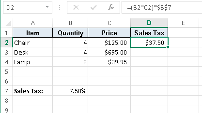
Figure 29-1:
Formula references to the sales tax cell should be absolute.

This formula uses relative cell references (B2 * C2) and also an absolute reference to the sales tax cell ($B$7). This formula can be copied to the cells below, and all of the references will be correct. For example, after copying the formula in cell D2, cell D3 contains this formula:

=(B3*C3)*$B$7


The references to the cells in columns B and C are adjusted, but the reference to cell B7 is not — which is exactly what you want.

Using mixed references

In a
mixed cell reference,
either the column part or the row part of a reference is absolute (and therefore doesn’t change when the formula is copied and pasted). Mixed cell references aren’t used often, but as you see in this tip, in some situations, using mixed references makes your job much easier.

Here are two examples of mixed references:

=$A1


=A$1


In the first example, the column part of the reference (A) is absolute, and the row part (1) is relative. In the second example, the column part of the reference is relative, and the row part is absolute.

Figure 29-2 shows a worksheet demonstrating a situation in which using mixed references is the best choice.

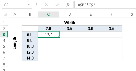
Figure 29-2:
Using mixed cell references.

The formulas in the table calculate the area for various lengths and widths of a rectangle. Here’s the formula in cell C3:

=$B3*C$2


Notice that both cell references are mixed. The reference to cell B3 uses an absolute reference for the column ($B), and the reference to cell C2 uses an absolute reference for the row ($2). As a result, this formula can be copied down and across, and the calculations are correct. For example, the formula in cell F7 is

=$B7*F$2


If C3 used either absolute or relative references, copying the formula would produce incorrect results.

Tip 30: Avoiding Error Displays in Formulas

Sometimes a formula returns an error, such as #REF! or #DIV/0!. Usually, you want to know when a formula error occurs so you can fix it. But in some cases, you might prefer to simply avoid displaying the error messages. Figure 30-1 shows an example.

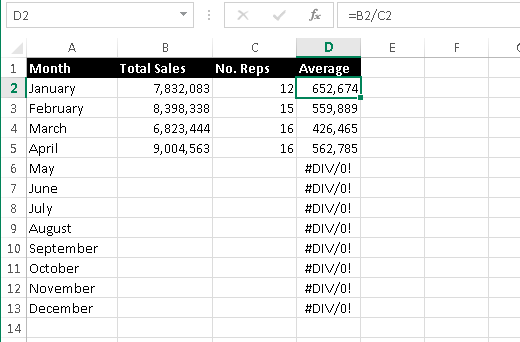
Figure 30-1:
The formulas in column D display an error if the data is missing.

Column D contains formulas that calculate the average sales volume. For example, cell D2 contains this formula:

=B2/C2


Using the IFERROR function

As you can see, the formula displays an error if the cells used in the calculation are empty. If you prefer to hide those error values, you can do so by using an IFERROR function. This function takes two arguments: The first argument is the expression that’s checked for an error, and the second is the value to return if the formula evaluates to an error.

The formula presented earlier can be rewritten as

=IFERROR(B2/C2,””)


As you see in Figure 30-2, when this formula is copied down the column, the result is a bit more visually pleasing.

By the way, you can put anything you like as the second argument for the IFERROR function. (It doesn’t have to be an empty string.) For example, you can make it a cell reference.

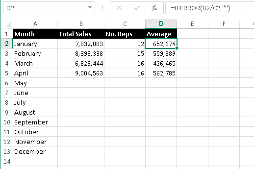
Figure 30-2:
Using an IFERROR function to hide error values.

The IFERROR function was introduced in Excel 2007, so it doesn’t work with earlier versions of Excel. If you plan to share your workbook with people who use Excel 2003 or earlier, you’ll need to use the ISERROR function — described next.

Using the ISERROR function

The ISERROR function is used with an IF function. For the example presented earlier, use this formula in cell D1:

=IF(ISERROR(B2/C2),””,B2/C2)


The ISERROR function returns TRUE if its argument evaluates to an error. In such a case, the IF function returns an empty string. Otherwise, the IF function returns the calculated value.

This method of avoiding an error display is a bit more complicated, and it’s also less efficient because the formula is actually evaluated two times if it doesn’t return an error. Therefore, unless you require compatibility with Excel 2003 or earlier versions, you should use the IFERROR functions.

Tip 31: Creating Worksheet-Level Names

Normally, when you name a cell or range, you can use that name in all worksheets in the workbook. For example, if you create a name, say
RegionTotal
, that refers to the cell M32 on Sheet1, you can use this name in any formula in any worksheet. This name is a workbook-level name (or a global name). By default, all cell and range names are workbook-level names.

Suppose that you have several worksheets in a workbook (one for each region) and you want to use the same name (such as
RegionTotal
) on each sheet. In this case, you need to create worksheet-level names (sometimes referred to as local names).

To define the worksheet-level name
RegionTotal
, activate the worksheet in which you want to define the name and choose Formulas⇒Defined Names⇒Define Name. The New Name dialog box then appears. In the Names field, enter the name in the Name field and use the Scope drop-down list to select the sheet in which the name is valid. Figure 31-1 shows a worksheet-level name being created.

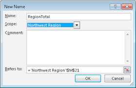
Figure 31-1:
Creating a worksheet-level name.

You can also create a worksheet-level name by using the Name box (located to the left of the Formula bar). Select the cell or range you want named, click in the Name box, and type the name, preceded by the sheet name and an exclamation point. Press Enter to create the name. Here’s an example of a worksheet-level name:

Sheet3!RegionTotal


If the worksheet name contains at least one space, enclose the worksheet name in apostrophes, like this:

‘Northwest Region’!RegionTotal


When you write a formula that uses a worksheet-level name on the sheet in which you defined it, you don’t need to include the worksheet name in the range name. (The Name box doesn’t display the worksheet name, either.) If you use the name in a formula on a
different
worksheet, however, you must use the entire name (sheet name, exclamation point, and name).