101 Excel 2013 Tips, Tricks and Timesavers (18 page)

=CEILING.MATH(A1,0.01)


To round down a dollar value, use the FLOOR.MATH function. The following formula, for example, rounds down the dollar value in cell A1 to the nearest penny (if cell A1 contains $12.421, the formula returns $12.42):

=FLOOR.MATH(A1,0.01)


To round up a dollar value to the nearest nickel, use this formula:

=CEILING.MATH(A1,0.05)


Using the INT and TRUNC functions

On the surface, the INT and TRUNC functions seem similar. Both convert a value to an integer. The TRUNC function simply removes the fractional part of a number. The INT function rounds down a number to the nearest integer, based on the value of the fractional part of the number.

In practice, INT and TRUNC return different results only when using negative numbers. For example, the following formula returns –14.0:

=TRUNC(-14.2)


The next formula returns –15.0 because –14.2 is rounded down to the next lower integer:

=INT(-14.2)


The TRUNC function takes an additional (optional) argument that’s useful for truncating decimal values. For example, the following formula returns 54.33 (the value truncated to two decimal places):

=TRUNC(54.3333333,2)


Rounding to n significant digits

In some situations, you may need to round a value to a particular number of significant digits. For example, you may want to express the value 1,432,187 in terms of two significant digits (that is, as 1,400,000). The value 84,356 expressed in terms of three significant digits is 84,300.

If the value is a positive number with no decimal places, the following formula does the job. This formula rounds the number in cell A1 to two significant digits. To round to a different number of significant digits, replace the 2 in this formula with a different number:

=ROUNDDOWN(A1,2-LEN(A1))


For non-integers and negative numbers, the solution is a bit trickier. The following formula provides a more general solution that rounds the value in cell A1 to the number of significant digits specified in cell A2. This formula works for positive and negative integers and non-integers:

=ROUND(A1,A2-1-INT(LOG10(ABS(A1))))


For example, if cell A1 contains 1.27845 and cell A2 contains 3, the formula returns 1.28000 (the value, rounded to three significant digits).

Tip 43: Converting Between Measurement Systems

You know the distance from New York to London in miles, but your European office needs the numbers in kilometers. What’s the conversion factor?

The Excel CONVERT function can convert between a variety of measurements in these categories:

→ Area

→ Distance

→ Energy

→ Force

→ Information

→ Magnetism

→ Power

→ Pressure

→ Speed

→ Temperature

→ Time

→ Volume (or liquid measure)

→ Weight and mass

The CONVERT function requires three arguments: the value to be converted, the from-unit, and the to-unit. For example, if cell A1 contains a distance expressed in miles, use this formula to convert miles to kilometers:

=CONVERT(A1,”mi”,”km”)


The second and third arguments are unit abbreviations, which are listed in the Help system. Some abbreviations are commonly used, but others aren’t. And, of course, you must use the
exact
abbreviation. Furthermore, the unit abbreviations are case-sensitive, so the following formula returns an error:

=CONVERT(A1,”Mi”,”km”)


The CONVERT function is even more versatile than it seems. When using metric units, you can apply a multiplier. In fact, the first example I presented uses a multiplier. The unit abbreviation for the third argument is
m,
for meters. I added the kilo-multiplier (
k
) to express the result in kilometers.

In some situations, the CONVERT function requires some creativity. For example, if you need to convert 100 km/hour into miles/sec, the formula requires two uses of the CONVERT function:

=CONVERT(100,”km”,”mi”)/CONVERT(1,”hr”,”sec”)


The CONVERT function has been significantly enhanced in Excel 2013 and supports dozens of new measurement units.

If you can’t find a particular unit that works with the CONVERT function, perhaps Excel has another function that will do the job. Table 43-1 lists some other functions that convert between measurement units.

Table 43-1:
Other Conversion Functions

* Function is new to Excel 2013.

Tip 44: Counting Nonduplicated Entries in a Range

In some situations, you may need to count the number of nonduplicated entries in a range. Figure 44-1 shows an example. Column A has a list of animals, and the goal is to count the number of different animals in the list. The formula in cell B2 returns 6, which is the number of nonduplicated animals. This formula (an array formula, by the way) is

=SUM(1/COUNTIF(A1:A10,A1:A10))


To adapt this formula to your own worksheet, just change both instances of A1:A10 to the range address that you’re working with.

When you enter an array formula, press Ctrl+Shift+Enter (not just Enter).

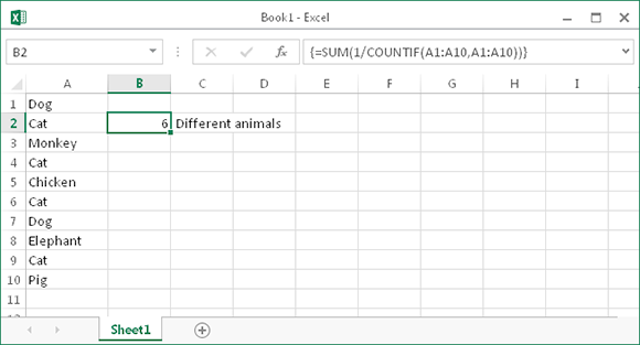
Figure 44-1:
Use an array formula to count the number of nonduplicated entries in a range.

This formula is one of those “Internet classics” that is passed around on various websites and newsgroups. Credit goes to David Hager, who first came up with the formula.

The preceding array formula works fine unless the range contains one or more empty cells. The following modified version of this array formula uses the IFERROR function to overcome this problem:

=SUM(IFERROR(1/COUNTIF(A1:A10,A1:A10),0))


The preceding formulas work with both values and text. If the range contains only numeric values or blank cells (but no text), you can use the following formula (which isn’t an array formula) to count the number of nonduplicated values:

=SUM(N(FREQUENCY(A1:A10,A1:A10)>0))


Tip 45: Using the AGGREGATE Function

One of the most versatile functions available in Excel is AGGREGATE, which was introduced in Excel 2010. You can use this multipurpose function to sum values, calculate an average, count entries, and more. What makes this function useful is that it can (optionally) ignore values in hidden rows and error values. In some cases, you can use AGGREGATE to replace a complex array formula.

The AGGREGATE function takes three arguments, but for some functions, an additional argument is required.

The first argument for the AGGREGATE function is a value between 1 and 19 that determines the type of calculation to perform. The calculation type, in essence, is one of Excel’s other functions. Table 45-1 contains a list of these values, with the function it mimics.

Table 45-1:
Values for the First Argument of the AGGREGATE Function

* Indicates a function that requires an additional (4th) argument.

The second argument for the AGGREGATE function is an integer between 0 and 7 that specifies how hidden cells and errors are handled. Table 45-2 summarizes these options.

Table 45-2:
Values for the Second Argument of the AGGREGATE Function

The third argument of the AGGREGGATE function is a range reference for the data to be aggregated.

The SUBTOTAL function always ignores data that is hidden, but only if the hiding is a result of filtering a table or contracting an outline. The AGGREGATE function works similarly, but also ignores data in rows that has been hidden manually. Note that this function does not ignore data in hidden columns. In other words, the AGGREGATE function was designed to work only with vertical ranges.