Antifragile: Things That Gain from Disorder (81 page)
Read Antifragile: Things That Gain from Disorder Online
Authors: Nassim Nicholas Taleb

Fragility has a left tail and, what is crucial, is therefore sensitive to perturbations of the left side of the probability distribution.
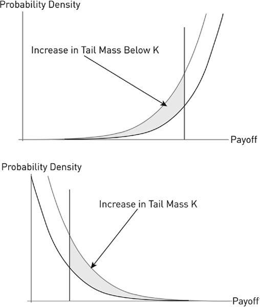
FIGURE 23
.
Definition of Fragility
(top graph): Fragility is the shaded area, the increase in the mass in left tail below a certain level K of the target variable in response to any change in parameter of the source variable—mostly the “volatility” or something a bit more tuned. We subsume all these changes in s
–
, about which later in the notes section (where I managed to hide equations).
For a
definition of antifragility
(bottom graph), which is not exactly symmetric, the
same mirror image for right tail plus robustness in left tail. The parameter perturbated is s
+
.
It is key that while we may not be able to specify the probability distribution with any precision, we can probe the response through heuristics thanks to the “transfer theorem” in Taleb and Douady (2012). In other words, we do not need to understand the future probability of events, but we can figure out the fragility to these events.
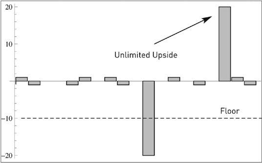
FIGURE 24
.
Barbell seen in time series space. Flooring payoffs while keeping upside.
A graphical expression of the barbell idea.
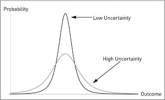
FIGURE 25
.
Case 1,
the Symmetric Case.
Injecting uncertainty into the system makes us move from one bell shape—the first, with narrow possible spate of outcomes—to the second, a lower peak but more spread out. So it causes an increase of both positive and negative surprises, both positive and negative Black Swans.
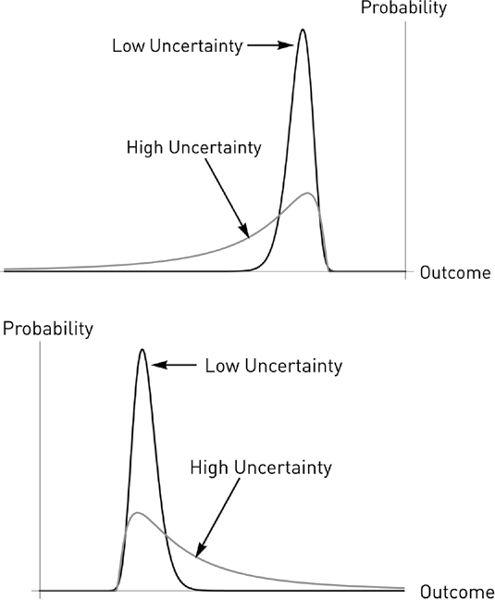
FIGURE 26
.
Case 2 (top):
Fragile.
Limited gains, larger losses. Increasing uncertainty in the system causes an augmentation of mostly (sometimes only) negative outcomes, just negative Black Swans. Case 3 (bottom):
Antifragile.
Increasing randomness and uncertainty in the system raises the probability of very favorable outcomes, and accordingly expand the expected payoff. It shows how discovery is, mathematically, exactly like an anti–airplane delay.
This note will also explain a “convex transformation.”
f
(
x
) is
exposure
to the variable
x. f
(
x
) can equivalently be called “payoff from
x,
” “exposure to
x,
” even “utility of payoff from
x
” where we introduce in
f
a utility function.
x
can be anything.
Example
:
x
is the intensity of an earthquake on some scale in some specific area,
f
(
x
) is the number of persons dying from it. We can easily see that
f
(
x
) can be made more predictable than
x
(if we force people to stay away from a specific area or build to some standards, etc.).
Example
:
x
is the number of meters of my fall to the ground when someone pushes me from height
x, f
(
x
) is a measure of my physical condition from the effect of the fall. Clearly I cannot predict
x
(who will push me, rather
f
(
x
)).
Example
:
x
is the number of cars in NYC at noon tomorrow,
f
(
x
) is travel time from point A to point B for a certain agent.
f
(
x
) can be made more predictable than
x
(take the subway, or, even better, walk).
Some people talk about
f
(
x
) thinking they are talking about
x.
This is the problem of the
conflation
of
event
and
exposure
. This error present in Aristotle is virtually ubiquitous in the philosophy of probability (say, Hacking).
One can become antifragile to
x
without understanding x, through convexity of
f
(
x
).
The answer to the question “what do you do in a world you don’t understand?” is, simply, work on the undesirable states of
f
(
x
).
It is often easier to modify
f
(
x
) than to get better knowledge of
x.
(In other words, robustification rather than forecasting Black Swans.)
Example
: If I buy an insurance on the market, here
x,
dropping more than 20 percent,
f
(
x
) will be independent of the part of the probability distribution of
x
that is below 20 percent and impervious to changes in its scale parameter. (This is an example of a barbell.)
FIGURE 27
.
Convex Transformation (f(x) is a convex function of x).
The difference between x and exposure to x. There is no downside risk in the second graph. The key is to modify f(x) in order to make knowledge of the properties of x on the left side of the distribution as irrelevant as possible. This operation is called convex transformation, nicknamed “barbell” here.
Green lumber fallacy:
When one confuses
f
(
x
) for another function
g
(
x
), one that has different nonlinearities.
More technically
: If one is antifragile to
x,
then the variance (or volatility, or other measures of variation) of
x
benefit
f
(
x
), since distributions that are skewed have their mean depend on the variance and when skewed right, their expectation increases with variance (the lognormal, for instance, has for mean a term that includes +½ σ
2
).
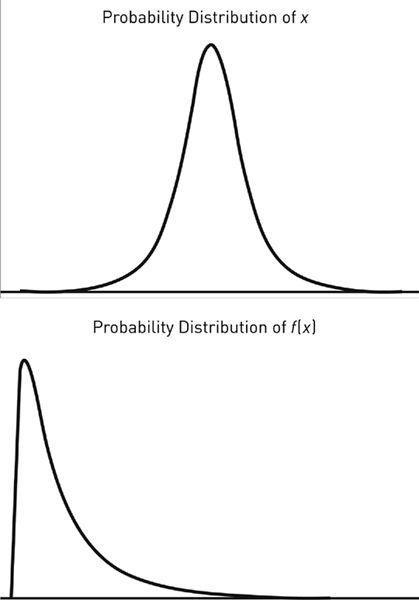
Further, the probability distribution of
f
(
x
) is markedly different from that of
x
, particularly in the presence of nonlinearities.
When
f
(
x
) is convex (concave) monotonically,
f
(
x
) is right (left) skewed.
When
f
(
x
) is increasing and convex on the left then concave to the right, the probability distribution of
f
(
x
) is thinner-tailed than that of
x
. For instance, in Kahneman-Tversky’s prospect theory, the so-called utility of changes in wealth is more “robust” than that of wealth.
Why payoff matters more than probability (technical):
Where
p
(
x
) is the density, the expectation, that is ∫
f
(
x
)
p
(
x
)
dx,
will depend increasingly on
f
rather than
p,
and the more nonlinear
f,
the more it will depend on
f
rather than
p
.
The idea is that tail events are not computable (in fat-tailed domains), but we can assess our exposure to the problem. Assume
f
(
x
) is an increasing function,
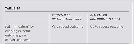
Table 10
connects the idea to the notion of the Fourth Quadrant.
