How We Know What Isn't So (4 page)
Read How We Know What Isn't So Online
Authors: Thomas Gilovich
Tags: #Psychology, #Developmental, #Child, #Social Psychology, #Personality, #Self-Help, #Personal Growth, #General

Judgment by representativeness is often valid and helpful because objects, instances, and categories that go together often do in fact share a resemblance. Many librarians fit the prototype of a librarian—after all, the prototype came from somewhere. Causes often resemble their effects: All else being equal, “bigger” effects require “bigger” causes, complex effects stem from complex causes, etc. It is the
overapplication
of representativeness that gets us into trouble. All else is not always equal. Not all librarians are prototypical; Some big effects (e.g., an epidemic) have humble causes (e.g., a virus) and some complex effects (e.g., the alteration of a region’s ecological balance) have simple causes (e.g., the introduction of a single pesticide).
It is easy to see how judgment by representativeness could contribute to the clustering illusion. In the case of coin flipping, one of the most salient features of a fair coin is the set of outcomes it produces—an approximate 50-50 split of heads and tails. In examining a sequence of coin flips, this 50-50 feature of the coin is automatically compared to the sequence of outcomes itself. If the sequence is split roughly 50-50, it strikes us as random because the outcome appears representative of a random generating process. A less even split is harder to accept. These intuitions are correct, but only in the long term. The law of averages (called the “law of large numbers” by statisticians) ensures that there will be close to a 50-50 split after a large number of tosses. After only a few tosses, however, even very unbalanced splits are quite likely. There is no “law of small numbers.”
The clustering illusion thus stems from a form of over-generalization: We expect the correct proportion of heads and tails or hits and misses to be present not only globally in a long sequence, but also locally in each of its parts. A sequence like the one shown previously with 8 hits in the first 11 shots does not look random because it deviates from the expected 50-50 split. In such a short sequence, however, such a split is not terribly unlikely.
Misperceptions of Random Dispersions
. The hot hand is not the only erroneous belief that stems from the compelling nature of the clustering illusion. People believe that fluctuations in the prices of stocks on Wall Street are far more patterned and predictable than they really are. A random series of changes in stock prices simply does not look random; it seems to contain enough coherence to enable a wily investor to make profitable predictions of future value from past performance. People who work in maternity wards witness streaks of boy births followed by streaks of girl births that they attribute to a variety of mysterious forces like the phases of the moon. Here too, the random sequences of births to which they are exposed simply do not look random.
The clustering illusion also affects our assessments of spatial dispersions. As noted earlier, people “see” a face on the surface of the moon and a series of canals on Mars, and many people with a religious orientation have reported seeing the likeness of various religious figures in unstructured stimuli such as grains of wood, cloud formations, even skillet burns. A particularly clear illustration of this phenomenon occurred during the latter stages of World War II, when the Germans bombarded London with their “vengeance weapons”—the V-1 buzz bomb and the V-2 rocket. During this “Second Battle of London,” Londoners asserted that the weapons appeared to land in definite clusters, making some areas of the city more dangerous than others.
9
However, an analysis carried, out after the war indicated that the points of impact of these weapons were randomly dispersed throughout London.
10
Although with time the Germans became increasingly accurate in terms of having a higher percentage of these weapons strike London, within this general target area their accuracy was sufficiently limited that any location was as likely to be struck as any other.
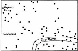
Still, it is hard not to empathize with those who thought the weapons fell in clusters. A random dispersion of events often does not look random, as
Figure 2.2
indicates. This figure shows the points of impact of 67 V-1 bombs in Central London.
11
Even after learning the results of the proper statistical analysis, the points do not look randomly dispersed. The lower right quadrant looks devastated and the upper left quadrant also looks rather hard hit; the upper right and lower left quadrants, however, appear to be relatively tranquil. We can easily imagine how the presence of special target areas could have seemed to Londoners to be an “irresistible product of their own experience.”
A close inspection of
Figure 2.2
sheds further light on why people “detect” order in random dispersions. Imagine
Figure 2.2
being bisected both vertically and horizontally, creating four quadrants of equal area. As already discussed, this results in an abundance of points in the upper-left and lower-right quadrants, and a dearth of points in the other two areas. In fact, the appropriate statistical test shows this clustering to be a significant departure from an independent, random dispersion.
*
In other words, when the dispersion of points is carved up in this particular way, non-chance clusters can be found. It is the existence of such clusters, no doubt, that creates the impression that the bombs did not fall randomly over London.
Figure 2.2
Points of Impact of 67 V-1 Bombs in Central London
But why carve the map this way? (Indeed, why conduct the statistical analysis only on the data from this particular area of London?) Why not bisect this figure with two diagonal lines? Bisected that way, there are no significant clusters.
The important point here is that with
hindsight
it is always possible to spot the most anomalous features of the data and build a favorable statistical analysis around them. However, a properly-trained scientist (or simply a wise person) avoids doing so because he or she recognizes that constructing a statistical analysis retrospectively capitalizes too much on chance and renders the analysis meaningless. To the scientist, such apparent anomalies merely suggest hypotheses that are subsequently tested on other,
independent
sets of data. Only if the anomaly persists is the hypothesis to be taken seriously.
Unfortunately, the intuitive assessments of the average person are not bound by these constraints. Hypotheses that are formed on the basis of one set of results are considered to have been proven by those very same results. By retrospectively and selectively perusing the data in this way, people tend to make too much of apparent anomalies and too often end up detecting order where none exists.
The main thrust of these examples, and the major point of this chapter, lies in the inescapable conclusion that our difficulty in accurately recognizing random arrangements of events can lead us to believe things that are not true—to believe something is systematic, ordered, and “real” when it is really random, chaotic, and illusory. Thus, one of the most fundamental tasks that we face in accurately perceiving and understanding our world—that of determining whether there is a phenomenon “out there” that warrants attention and explanation—is a task that we perform imperfectly.
Furthermore, once we suspect that a phenomenon exists, we generally have little trouble explaining
why
it exists or what it means. People are extraordinarily good at ad hoc explanation. According to past research, if people are erroneously led to believe that they are either above or below average at some task, they can explain either their superior or inferior performance with little difficulty.
12
If they are asked to account for how a childhood experience such as running away from home could lead during adulthood to outcomes as diverse as suicide or a job in the Peace Corps, they can do so quite readily and convincingly.
13
To live, it seems, is to explain, to justify, and to find coherence among diverse outcomes, characteristics, and causes. With practice, we have learned to perform these tasks quickly and effectively.
A dramatic illustration of our facility with ad hoc explanation comes from research on split-brain patients. In nearly all of these patients, language ability is localized in the left cerebral hemisphere, as it is in most people. The one difference between split-brain patients and other individuals is that communication between the two hemispheres is prevented in the split-brain patient because of a severed corpus callosum. Imagine, then, that two different pictures are presented to the two hemispheres of a split-brain patient. A picture of a snow-filled meadow is presented to the nonverbal right hemisphere (by presenting it in the left visual field). Simultaneously, a picture of a bird’s claw is presented to the verbal left hemisphere (by presenting it in the right visual field). Afterwards, the patient is asked to select from an array of pictures the one that goes with the stimuli he or she had just seen.
What happens? The usual response is that the patient selects two pictures. In this instance, the person’s left hand (controlled by the right hemisphere) might select a shovel to go with the snow scene originally presented to the right hemisphere. At the same time, the right hand (controlled by the left hemisphere) might select a picture of a chicken to go with the claw originally presented to the left hemisphere. Both responses fit the relevant stimulus because the response mode—pointing—is one that can be controlled by each cerebral hemisphere. The most interesting response occurs when the patient is asked to explain the choices he or she made. Here we might expect some difficulty because the verbal response mode is controlled solely by the left hemisphere. However, the person generally provides an explanation without hesitation: “Oh, that’s easy. The chicken claw goes with the chicken and you need a shovel to clean out the chicken shed.”
14
Note that the real reason the subject pointed to the shovel was not given, because the snow scene that prompted the response is inaccessible to the left hemisphere that must fashion the verbal explanation. This does not stop the person from giving a “sensible” response: He or she examines the relevant output and invents a story to account for it. It is as if the left hemisphere contains an explanation module along with, or as part of, its language center—an explanation module that can quickly and easily make sense of even the most bizarre patterns of information.
15
This work has important implications for the ideas developed in this chapter. It suggests that once a person has (mis)identified a random pattern as a “real” phenomenon, it will not exist as a puzzling, isolated fact about the world. Rather, it is quickly explained and readily integrated into the person’s pre-existing theories and beliefs. These theories, furthermore, then serve to bias the person’s evaluation of new information in such a way that the initial belief becomes solidly entrenched. Indeed, as the astute reader has probably discerned, the story of our research on the hot hand is only partly a story about the misperception of random events. As the common response to our research makes clear, it is also a story about how people cling tenaciously to their beliefs in the face of hostile evidence. In Chapter 4 we return to the subject of how people’s theories and expectations influence their evaluation of evidence.
An important lesson taught in nearly every introductory statistics course is that when two variables are related, but imperfectly so, extreme values on one of the variables tend to be matched by less extreme values on the other. This is the regression effect. The heights of parents and children are related, but the relationship is not perfect—it is subject to variability and fluctuation. The same is true of a student’s grades in high school and in college, a company’s profits in consecutive years, a musician’s performance from concert to concert, etc. As a consequence, very tall parents tend to have tall children, but not as tall (on average) as they are themselves; high school valedictorians tend to do well in college, but not as well (on average) as they did in high school; a company’s disastrous years tend to be followed by more profitable ones, and its banner years by those that are less profitable. When one score is extreme, its counterpart tends to be closer to the average. It is a simple statistical fact.
*
The concept of statistical regression is not terribly difficult, and most people who take a statistics course can learn to answer correctly the standard classroom questions about the heights of fathers and sons, the IQs of mothers and daughters, and the SAT scores and grade point averages of college students. People have more difficulty, however, acquiring a truly general and deep understanding that whenever
any
two variables are imperfectly correlated, extreme values of one of the variables are matched, on the average, by less extreme values of the other. Without this deeper understanding, people encounter two problems when they venture out in the world and deal with less familiar instances of regression.