The Bell Curve: Intelligence and Class Structure in American Life (102 page)
Read The Bell Curve: Intelligence and Class Structure in American Life Online
Authors: Richard J. Herrnstein,Charles A. Murray
Tags: #History, #Science, #General, #Psychology, #Sociology, #Genetics & Genomics, #Life Sciences, #Social Science, #Educational Psychology, #Intelligence Levels - United States, #Nature and Nurture, #United States, #Education, #Political Science, #Intelligence Levels - Social Aspects - United States, #Intellect, #Intelligence Levels

The size of
R
2 tells something about the strength of the logistic relationship between the dependent variable and the set of independent variables, but it also depends on the composition of the sample, as do correlation coefficients in general. Even an inherently strong relationship can result in low values of
R
2 if the data points are bunched in various ways, and relatively noisy relationships can result in high values if the sample includes disproportionate numbers of outliers. For example, one of the smallest
R
2 in the following analyses, only .017, is for white men out of the labor force for four weeks or more in 1989. Apart from the distributional properties of the data that produce this low
R
2, a rough common-sense meaning to keep in mind is that the vast majority of NLSY white men were in the labor force even though they had low IQs or deprived socioeconomic backgrounds. But the parameter for zAFQT in that same equation is significant beyond the .001 level and large enough to make a big difference in the probability that a white male would be out of the labor force. This illustrates why we therefore consider the regression coefficients themselves (and their associated
p
values) to suit our analytic purposes better than
R
2, and that is why those are the ones we relied on in the text.
The standard independent variables, described in Appendix 2, are zAFQT89, the 1989 scoring of the AFQT; zSES, the socioeconomic background of the NLSY subjects; and zAge, based on the age of the NLSY subjects as of December 31, 1990. All are expressed as standard scores with a mean of 0 and a standard deviation of 1.
All dependent variables are binary. The coefficients are parameter estimates when the dependent variable = “yes.” The linear logistic model has the form
logit(p) = log(p/(1−p)) = α + ß′x
where α is the intercept parameter and ß is the vector of slope parameters for a vector of independent variables x. Take as an example the first set of results presented subsequently, involving poverty. Suppose you want to know the probability that a person is under the poverty line in 1989 (Poverty = “Yes”), stipulating that the person in question has an IQ (zAFQT) 1.5 standard deviations below the mean, socioeconomic background (zSES) .3 standard deviation above the mean, and is exactly of mean age. Using the parameters in the basic analysis for poverty rounded to four decimal places, and a computationally convenient re-expression of
p,
the probability is computed as follows:
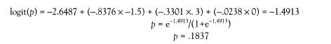
The probability we set out to compute is 18.37 percent.
“The High School Sample” consists of those who received a high school diploma through the normal route (not a GED) and reported exactly twelve years of education as of the 1990 interview.
“The College Sample” consists of those who completed a bachelor’s degree and reported exactly sixteen years of education as of the 1990 interview.
The software used for the analyses is JMP Version 3, by SAS Institute Inc. JMP treats nominal independent variables differently from other major software packages such as SAS and SPSS. In those packages, a parameter for a nominal variable represents the difference between that level of the nominal variable and an omitted level serving as a reference group. In JMP, a parameter represents the difference of a given level from the average over all levels of the nominal variable. The implied parameter for the remaining level is the negative sum of the other levels (i.e., the parameters sum to zero over all the effect levels). For example, suppose Race were being used as a nominal variable, with categories of Black, Latino, and White. In the JMP printout, the coefficients would appear as
| Race[Black-White] | x1 |
| Race [Latino-White] | x2 |
The order is determined by the alphabetical order of the categories. In this case, the coefficient x1 applies to blacks, x2 to Latinos. The implied White coefficient is −1 × (x1 + x2). In the case of a binary independent variable such as Sex, the printout would show a single line
Sex [Female-Male] x1
which applies to females. The coefficient for Male equals −x1.
DEPENDENT VARIABLE:
Under the official poverty line in 1989.
SAMPLE RESTRICTIONS:
Excludes those who reported they were out of the labor force because they were in school in either the 1989 or 1990 interviews.
Whole-Model Test
| Source | DF | -LogLikelihood | ChiSquare | Prot>ChiSq |
| Model | 3 | 90.94009 | 181.8802 | 0.000000 |
| Error | 3363 | 784.40179 | | |
| C Total | 3366 | 875.34188 | | |
| | RSquare (U) | 0.1039 | | |
| | Observations | 3367 | |
Parameter Estimates
| Term | Estimate | Std Error | ChiSquare | Prob>ChiSq |
| Intercept | −2.6487288 | 0.0768803 | 1187 | 0.0000 |
| zAFQT89 | −0.8376338 | 0.0935061 | 80.25 | 0.0000 |
| zSES | −0.3300720 | 0.0900996 | 13.42 | 0.0002 |
| zAge | −0.0238375 | 0.0723735 | 0.11 | 0.7419 |
Whole-Model Test
| Source | DF | -LogLikelihood | ChiSquare | Prob>ChiSq |
| Model | 3 | 22.01811 | 44.03622 | 0.000000 |
| Error | 1232 | 325.26939 | | |
| C Total | 1235 | 347.28750 | | |
| | RSquare (U) | 0.0634 | | |
| | Observations | 1236 | |
Parameter Estimates
| Term | Estimate | Std Error | ChiSquare | Prob>ChiSq |
| Intercept | −2.7237775 | 0.1290286 | 445.63 | 0.0000 |
| zAFQT89 | −0.8267293 | 0.1627358 | 25.81 | 0.0000 |
| zSES | −0.3619703 | 0.1499855 | 5.82 | 0.0158 |
| zAge | +0.1049227 | 0.1094603 | 0.92 | 0.3378 |
The College Sampk:
Omitted. Only six persons in the cross-sectional College Sample were in poverty.
Whole-Model Test
| Source | DF | -LogLikelihood | ChiSquare | Prob>ChiSq |
| Model | 3 | 17.14553 | 34.29106 | 0.000000 |
| Error | 786 | 179.84999 | | |
| C Total | 789 | 196.99552 | | |
| | RSquare (U) | 0.0870 | | |
| | Observations | 790 |
Parameter Estimates
| Term | Estimate | Std Error | ChiSquare | Prob>ChiSq |
| Intercept | −2.7732817 | 0.1646023 | 283.87 | 0.0000 |
| zAFQT89 | −0.6437797 | 0.2140132 | 9.05 | 0.0026 |
| zSES | −0.3910629 | 0.2020317 | 3.75 | 0.0529 |
| zAge | −0.3338674 | 0.1587605 | 4.42 | 0.0355 |
Whole-Model Test
| Source | DF | -LogLikelihood | ChiSquare | Prob>ChiSq |
| Model | 3 | 8.07114 | 16.14228 | 0.001060 |
| Error | 211 | 135.77658 | | |
| C Total | 214 | 143.84772 | | |
| | RSquare (U) | 0.0561 | | |
| | Observations | 215 | |
Parameter Estimates
| Term | Estimate | Std Error | ChiSquare | Prob>ChiSq |
| Intercept | −0.7449132 | 0.1713794 | 18.89 | 0.0000 |
| zAFQT89 | −0.6722121 | 0.2277019 | 8.72 | 0.0032 |
| zSES | −0.1597461 | 0.1952709 | 0.67 | 0.4133 |
| zAge | −0.1524315 | 0.1530986 | 0.99 | 0.3194 |
DEPENDENT VARIABLE:
Permanently dropped out of high school.
SAMPLE RESTRICTIONS:
Excludes those who obtained a GED.
Whole-Model Test
| Source | DF | -LogLikelihood | ChiSquare | Prob>ChiSq |
| Model | 3 | 393.8978 | 787.7956 | 0.000000 |
| Error | 3568 | 779.9904 | | |
| C Total | 3571 | 1173.8882 | | |
| | RSquare (U) | 0.3355 | | |
| | Observations | 3572 | |
Parameter Estimates
| Term | Estimate | Std Error | ChiSquare | Prob>ChiSq |
| Intercept | −2.85322606 | 0.0939659 | 922.00 | 0.0000 |
| zAFQT89 | −1.72295934 | 0.1028145 | 280.83 | 0.0000 |
| zSES | −0.64776232 | 0.0896658 | 52.19 | 0.0000 |
| zAge | +0.05695640 | 0.0688286 | 0.68 | 0.4079 |
Whole-Model Test
| Source | DF | -LogLikelihood | ChiSquare | Prob>ChiSq |
| Model | 4 | 399.9876 | 799.9751 | 0.000000 |
| Error | 3567 | 773.9006 | | |
| C Total | 3571 | 1173.8882 | | |
| | RSquare (U) | 0.3407 | | |
| | Observations | 3572 | |
Parameter Estimates
| Term | Estimate | Std Error | ChiSquare | Prob>ChiSq |
| Intercept | −2.9143231 | 0.1029462 | 801.41 | 0.0000 |
| zAFQT89 | −1.8937642 | 0.1188518 | 253.89 | 0.0000 |
| zSES | −0.9402389 | 0.1250634 | 56.52 | 0.0000 |
| zAge | +0.0522667 | 0.0682755 | 0.59 | 0.4440 |
| zAFQT89*zSES | −0.4133224 | 0.1187879 | 12.11 | 0.0005 |
DEPENDENT VARIABLE:
Received a GED instead of a high school diploma.
SAMPLE RESTRICTIONS:
Excludes those who obtained neither a high school diploma nor a GED.
Whole-Model Test
| Source | DF | -LogLikelihood | ChiSquare | Prob>ChiSq |
| Model | 3 | 72.06475 | 144.1295 | 0.000000 |
| Error | 3490 | 915.28145 | | |
| C Total | 3493 | 987.34620 | | |
| | RSquare (U) | 0.0730 | | |
| | Observations | 3494 | |