Understanding Sabermetrics (29 page)
Read Understanding Sabermetrics Online
Authors: Gabriel B. Costa,Michael R. Huber,John T. Saccoma

The closer to 1 the value of
r
2
, the better the fit of the data to a simple linear regression model. Further, most current statistical programs provide the
r
2
value as part of the descriptive statistics output.
r
2
, the better the fit of the data to a simple linear regression model. Further, most current statistical programs provide the
r
2
value as part of the descriptive statistics output.
Rather than try to find one variable which can accurately predict another, let’s attempt to build a model which takes as its input several independent variables (
x
i
) and then predicts one dependent variable
y
. We will add up the independent variables (multiplied by different coefficients) and then create a model. For example, perhaps runs batted in can be predicted by using home runs, triples, and doubles. We assign a variable to each independent variable and our general additive multiple regression model becomes
where
x
1
corresponds to the number of home runs in a season,
x
2
corresponds to triples, and
x
3
are doubles. One might believe that a high number of extra-base hits correlates to a high number of RBIs. Let’s see if it’s true. There is still some error (
ε
) associated with this method. All of the independent variables appear linearly in this expression. This is the simplest multiple regression model. The dependent variable
y
is a linear function and we get a deviation from the expression by some amount known as the error. Notice that there is no interaction among the independent variables. Other multiple regression models exist which offer no interaction or complete interaction among the variables. For example,
 is a model which is now nonlinear but has no interaction between
x
1
and
x
2
. On the other hand,
shows interaction between and and is thus nonlinear (we could also add a term which has x
1
2
or x
2
2
if desirable). Further, the powers of each variable need not be integers. Nonlinear multiple regression models can be very complicated, and we will not explore them further in this discussion.
x
i
) and then predicts one dependent variable
y
. We will add up the independent variables (multiplied by different coefficients) and then create a model. For example, perhaps runs batted in can be predicted by using home runs, triples, and doubles. We assign a variable to each independent variable and our general additive multiple regression model becomes
y
=
β
0
+ β
1
x
1
+
β
2
x
2
+
β
3
x
3
+
ε
,
x
1
corresponds to the number of home runs in a season,
x
2
corresponds to triples, and
x
3
are doubles. One might believe that a high number of extra-base hits correlates to a high number of RBIs. Let’s see if it’s true. There is still some error (
ε
) associated with this method. All of the independent variables appear linearly in this expression. This is the simplest multiple regression model. The dependent variable
y
is a linear function and we get a deviation from the expression by some amount known as the error. Notice that there is no interaction among the independent variables. Other multiple regression models exist which offer no interaction or complete interaction among the variables. For example,

x
1
and
x
2
. On the other hand,
y =
β
0
+
β
1
x
1
+
β
2
x
2
+
β
3
x
1
x
2
+
ε
1
2
or x
2
2
if desirable). Further, the powers of each variable need not be integers. Nonlinear multiple regression models can be very complicated, and we will not explore them further in this discussion.
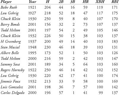
Table 12.4 Top extra-base hits leaders in a single season
As an example, there have only been fifteen times when a major league player has had 100 or more extra-base hits in a season. The first to do it was Babe Ruth in 1921, and his record of 119 extra-base hits in a single season still stands. Amazingly, four occurrences sprung out of the 2001 season. Just below this extraordinary listing of players are eight occurrences of 99 extra-base hits, including twice by Babe Ruth. Carlos Delgado is also one of the “not-quite-100” extra-base-hit players. Suppose we wished to calculate how many RBIs Carlos Delgado should have had in 2004, given his extra-base hit data. Let’s compare his statistics to those 15 best extra-base hit seasons. In Table 13.4 (on page 125) we list the players.
In trying to predict the number of runs batted in, we determine that the intercept,
β
0
, should equal 74.509, and the other three coefficients are as follows:
β
1
= 0.612,
β
2
= 1.765, and
β
3
= 0.704. Putting this all together, the prediction for runs batted in becomes
β
0
, should equal 74.509, and the other three coefficients are as follows:
β
1
= 0.612,
β
2
= 1.765, and
β
3
= 0.704. Putting this all together, the prediction for runs batted in becomes
RBIs = 74.509 + 0.612 × 2B + 1.765 × 3B + 0.704 × HR.
If we substitute Babe Ruth’s 1921 totals into the equation, we find that he should have had 74.509 + 0.612 × 44 + 1.765 × 16 + 0.704 × 59 = 171 RBIs, which is exactly his actual 1921 total of 171. Todd Helton’s 2001 season also predicts an RBI total of 146, his actual amount. What about Carlos Delgado? Based upon this multiple regression, his predicted RBI total should have been 140, which is within three of his actual total of 137.
Notice that the RBI equation listed above predicts 74 runs batted in, even if the player has no extra-base hits (substitute a zero in for the number of doubles, triples, and home runs). Also, the higher the value of the variable for the data sets, the less impact the coefficient has. Notice that the average number of doubles is higher than the average number of home runs for our 100+ extra-base hit sluggers. The average number of triples is much lower. So, the coefficients for triples is higher than that for home runs, which is slightly higher than that for doubles.
Suppose we had tried to model RBIs based solely on the number of extra-base hits (predict the last column of Table 12.4 using the second-to-last column only). Two scatter plots of extra-base hits versus runs batted in are shown in Figure 12.4 and Figure 12.5, along with a trend line (we used a simple linear regression model). In Figure 12.4, we use only those data sets corresponding to at least 100 extra-base hits. In Figure 12.5, we include all data corresponding to 90 or more extra-base hits in a season.
This scatter plot’s trend line has an
r
2
value of only 0.0997, which is not valuable. By using a multiple regression model on the data in Table 12.4, the
r
2
value increases to almost 24 percent (still not that good). However, when more data points are used (for example, when using the top 62 occurrences which equate to the seasons in which a batter had at least 90 extra-base hits), the
r
2
value increases to about 33 percent.
r
2
value of only 0.0997, which is not valuable. By using a multiple regression model on the data in Table 12.4, the
r
2
value increases to almost 24 percent (still not that good). However, when more data points are used (for example, when using the top 62 occurrences which equate to the seasons in which a batter had at least 90 extra-base hits), the
r
2
value increases to about 33 percent.
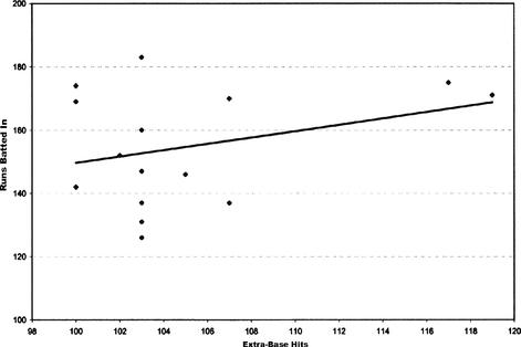
Figure 12.4 Scatterplot of extra-base hits versus runs batted in, top 15
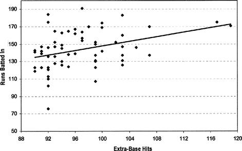
Figure 12.5 Scatterplot of extra-base hits versus runs batted in, top 62
Many fans may argue that more is involved in predicting RBIs. Perhaps that is true. Perhaps we should use a nonlinear regression model. Or, perhaps we should use other variables, such as split statistics. For example, what is a batter’s chance of driving in a run when runners are in scoring position? The above regression model does not take into account any runners being on base. Therefore, the only way a run will be batted in with no one on base is if the batter hits a home run and drives himself in. With the recent availability of data on the Internet, we could gather information about how many times a batter steps up to the plate with runners on base. That information could be factored into a regression model. The more data we wish to use as independent variables, the more complicated the model will become.
There are data sets that fit regression lines in a better way. Let’s consider runs scored by a team in a season. The table below shows the runs scored, with on-base percentage (OBP), slugging percentage (SLG) and the popular on-base plus slugging percentage (OPS).
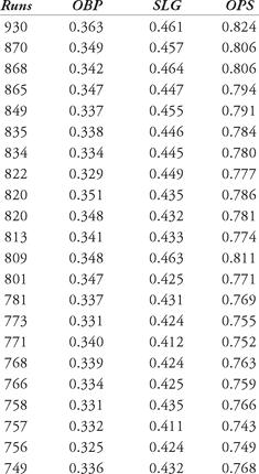
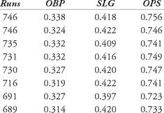
Table 12.5 Offensive data, 2006
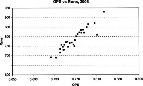
Let’s try to fit both a single-variable linear regression and a multi-variable linear regression equation to this set of data. First, we show a scatter plot of the data (OPS versus runs scored) in Figure 12.6. The data appears to exhibit a trend: as the OPS of a team increases, the number of runs scored also increases.
Other books
The Furies of Rome by Robert Fabbri
Yvvaros: The Digital Frontier by Alex Mulder
A Dragon's Bond by Johnson, S.B.
Pride and Prejudice (Clandestine Classics) by Jane Austen, Amy Armstrong
The Time of the Ghost by Diana Wynne Jones
Tales of Sin & Fury, Part 1 by Sonia Paige
Messed Up by Molly Owens
Decline (Declan Reede: The Untold Story #1) by Michelle Irwin
