X and the City: Modeling Aspects of Urban Life (50 page)
Read X and the City: Modeling Aspects of Urban Life Online
Authors: John A. Adam

(Hint: integrate by parts twice.)
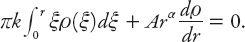
Now we proceed to look at some more specific city models. We set
γ
= 2 in “Axiom” VI and write equation (17.4) in terms of the population density
ρ
(
r
) to obtain
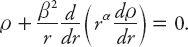
If we perform a differentiation and define
β
2
=
A
/π
k
, then we have
This expression can be rearranged in the form
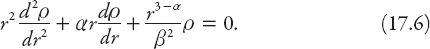
This equation is related to the well-known
Bessel equation
of order , namely.
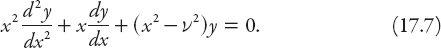
The constantmay take on any value, but is often an integer. A bounded solution to this equation satisfying the condition
y
′(0) = 1 is
y
=
J
v
(
x
), where
J
v
(
x
) is a Bessel function of the first kind of order. Consequently, the corresponding solution of equation (17.6) can be shown to be

In this expression
ρ
(0) is the central population density and= |(1 −
α
)/(3 −
α
)|. It will be left as an exercise for the reader to verify this result. Note that if
α
= 3, the original differential equation (17.6) reduces to Euler’s equation, solutions for which may be found by seeking them in the form
ρ
(
r
) ∝
r
m
and solving the resulting quadratic equation for
m
. Only solutions for which the real part of
m
is positive will be appropriate for a city containing the origin, but for an annular city, all solutions are in principle permitted.
Exercise:
Verify by direct construction that (17.8) is a solution to (17.6).
(Hint: let
ρ
(
r
) =
r
(1−
α
)/2
z
(
r
) and then make a change of independent variable,
t
=
r
(3−
α
)/2
.)
Such idealized “cities” can be referred to as “Bessel cities” for obvious reasons. When
α
= 1, the solution (17.8) reduces to the simple form
ρ
(
r
) =
ρ
(0)
J
0
(
r
/
β
), and when
α
= 2 the solution is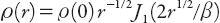 . From the definition of housing rental the corresponding expressions for
P
(
r
) are proportional to the squares of these solutions; they are illustrated in
Figure 17.2
. The model for
α
= 2 has the disadvantage that, unlike the case for
α
= 1, the gradients
ρ
′(0) and
P
′(0) at the center are not zero. While this is not a
major problem, this model does not have these “nice” properties enjoyed by the other one.
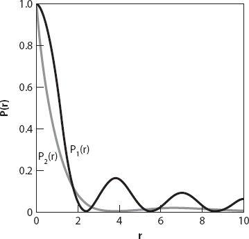
Figure 17.2.
P
1
(
r
) (solid line) is the square of the solution (17.8) for
α
= 1,
ρ
0
= 1, and
β
= 1 (for simplicity).
P
2
(
r
) (gray line) is the square of the solution (17.8) for
α
= 2,
ρ
0
= 1, and
β
= 1.