101 Excel 2013 Tips, Tricks and Timesavers (23 page)

The previous section describes how to perform simple mathematical transformations on a range of numeric data. This tip describes the much more versatile method of transforming data (numerical or text) by using temporary formulas.

Figure 57-2 shows a worksheet with names in column A. These names are in all uppercase letters, and the goal is to convert them to proper case (only the first letter of each name is uppercase).

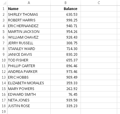
Figure 57-2:
The goal is to transform the names in column A to proper case.

Follow these steps to transform the data in column A:

1.
Create a temporary formula in an unused column.

For this example, enter this formula in cell C2:

=PROPER(A2)

2.
Copy the formula down the column to accommodate all cells to be transformed.

3.
Select the formula cells (in column C).

4.
Press Ctrl+C.

5.
Select the original data cells (in column A).

6.
Choose Home⇒Clipboard⇒Paste⇒Paste Values (V).

The original data is replaced with the transformed data (see Figure 57-3).

7.
Press Esc to cancel Copy mode.

8.
When you’re satisfied that the transformation happened as you intended, you can delete the temporary formulas in column C.

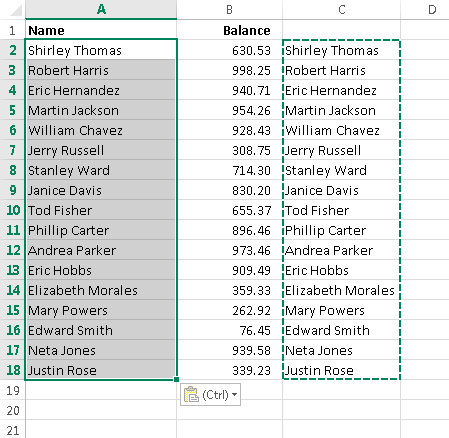
Figure 57-3:
The formula results from column C replace the original data in column A.

You can adapt this technique for just about any type of data transformation you need. The key, of course, is constructing the proper transformation formula in Step 1.

Tip 58: Creating a Drop-Down List in a Cell

Most Excel users probably assume that some advanced feature (such as a VBA macro) is required to display a drop-down list in a cell. But it’s not. You can easily display a drop-down list in a cell — no macros required.

Figure 58-1 shows an example. Cell B2, when selected, displays a down arrow. Click the arrow, and you get a list of items (in this case, month names). Click an item, and it appears in the cell. The drop-down list can contain text, numeric values, or dates. Your formulas, of course, can refer to cells that contain a drop-down list. The formulas always use the value that’s currently displayed.

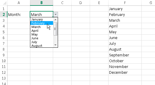
Figure 58-1:
Creating a drop-down list in a cell is easy and doesn’t require macros.

The trick to setting up a drop-down list is to use the data validation feature. The following steps describe how to create a drop-down list of items in a cell:

1.
Enter the list of items in a range.

In this example, the month names are in the range F1:F12.

2.
Select the cell that will contain the drop-down list (cell B2, in this example).

3.
Choose Data⇒Data Tools⇒Data Validation.

4.
In the Data Validation dialog box, click the Settings tab.

5.
In the Allow drop-down list, select List.

6.
In the Source box, specify the range that contains the items.

In this example, the range is E1:E12.

7.
Make sure that the In-Cell Dropdown option is checked (see Figure 58-2) and click OK.

If your list is short, you can avoid Step 1. Rather, just type your list items (separated by commas) in the Source box in the Data Validation dialog box.

If you plan to share your workbook with others who use Excel 2007 or earlier, make sure that the list is on the same sheet as the drop-down list. Alternatively, you can put the list on any sheet, as long as it’s a named range. For example, you can choose Formulas⇒Defined Names⇒Define Name to define the name
MonthNames
for E1:E12. Then, in the Data Validation dialog box, enter
=MonthNames
in the Source box.

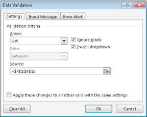
Figure 58-2:
Using the Data Validation dialog box to create a drop-down list.

Tip 59: Comparing Two Ranges by Using Conditional Formatting

A common task is comparing two lists of items to identify differences between the two lists. Doing it manually is far too tedious and error-prone, but Excel can make it easy. This tip describes a method that uses conditional formatting.

Figure 59-1 shows an example of two multicolumn lists of names. Applying conditional formatting can make the differences in the lists become immediately apparent. These list examples contain text, but this technique also works with numeric data.

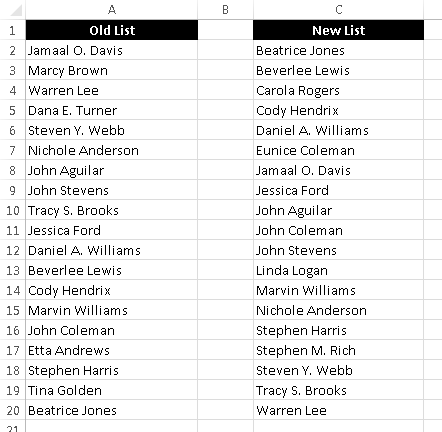
Figure 59-1:
You can use conditional formatting to highlight the differences in these two ranges.

The first list is in A2:A20, and this range is named
OldList
. The second list is in C2:C20, and the range is named
NewList
. The ranges were named by using the Formulas⇒Defined Names⇒Define Name command. Naming the ranges isn’t necessary, but it makes them easier to work with.

Start by adding conditional formatting to the old list:

1.
Select the cells in the
OldList
range.

2.
Choose Home⇒Conditional Formatting⇒New Rule to display the New Formatting Rule dialog box.

3.
In the New Formatting Rule dialog box, click the option labeled Use a Formula to Determine Which Cells to Format.

4.
Enter this formula in the dialog box (see Figure 59-2):

=COUNTIF(NewList,A2)=0


When using this technique with your own data, substitute the actual range address (or name) for NewList, and substitute the address of the top left selected cell for A2.

5.
Click the Format button and specify the formatting to apply when the condition is true.

A different fill color is a good choice.

6.
Click OK.

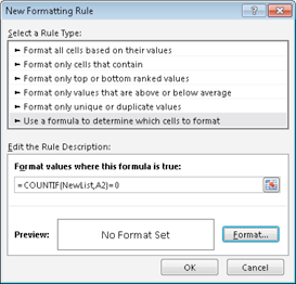
Figure 59-2:
Applying conditional formatting.

The cells in the
NewList
range use a similar conditional formatting formula.

1.
Select the cells in the
NewList
range.

2.
Choose Home⇒Conditional Formatting⇒New Rule to display the New Formatting Rule dialog box.

3.
In the New Formatting Rule dialog box, click the option labeled Use a Formula to Determine Which Cells to Format.

4.
Enter this formula in the dialog box:

=COUNTIF(OldList,C2)=0


When using this technique with your own data, substitute the actual range address (or name) for OldList, and substitute the address of the top left selected cell for C2.

5.
Click the Format button and specify the formatting to apply when the condition is true (a different fill color).

6.
Click OK.

Figure 59-3 shows the result. Names that are in the old list but not in the new list are highlighted. In addition, names in the new list that aren’t in the old list are highlighted in a different color. Names that aren’t highlighted appear in both lists.

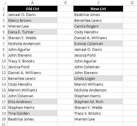
Figure 59-3:
Conditional formatting causes differences in the two lists to be highlighted.

Both of these conditional-formatting formulas use the COUNTIF function. This function counts the number of times a particular value appears in a range. If the formula returns 0, it means that the item doesn’t appear in the range. Therefore, the conditional formatting kicks in and the cell’s background color is changed.