The Bell Curve: Intelligence and Class Structure in American Life (96 page)
Read The Bell Curve: Intelligence and Class Structure in American Life Online
Authors: Richard J. Herrnstein,Charles A. Murray
Tags: #History, #Science, #General, #Psychology, #Sociology, #Genetics & Genomics, #Life Sciences, #Social Science, #Educational Psychology, #Intelligence Levels - United States, #Nature and Nurture, #United States, #Education, #Political Science, #Intelligence Levels - Social Aspects - United States, #Intellect, #Intelligence Levels

We still lack a convenient way of expressing where people are in that distribution. What does it mean to say that two different students are, say, 6 inches different in height. How “big” is a 6-inch difference? That brings us back to the standard deviation.
When it comes to high school students, you have a good idea of how big a 6-inch difference is. But what does a 6-inch difference mean if you are talking about the height of elephants? About the height of cats? It depends. And the things it depends on are the average height and how much height varies among the things you are measuring. A
standard deviation
gives you a way of taking both the average and that variability into account, so that “6 inches” can be expressed in a way that means the same thing for high school students relative to other high school students, elephants relative to other elephants, and cats relative to other cats.
Suppose that your high school class consisted of just two people who were 66 inches and 70 inches. Obviously, the average is 68 inches. Just as obviously, one person is 2 inches shorter than average, one person is 2 inches taller than average. The standard deviation is a kind of average of the differences from the mean—2 inches, in this example. Suppose you add two more people to the class, one who is 64 inches and the other who is 72 inches. The mean hasn’t changed (the two new people balance each other off exactly). But the newcomers are each 4 inches different from the average height of 68 inches, so the standard deviation, which measures the spread, has gotten bigger as well. Now two people are 4 inches different from the average and two people are 2 inches different from the average. That adds up to a total 12 inches, divided among four persons. The simple average of these differences from the mean is 3 inches (12 ÷ 4), which is almost (but not quite) what the standard deviation is. To be precise, the standard deviation is calculated by squaring the deviations from the mean, then summing them, then finding their average, then taking the square root of the result. In this example, two people are 4 inches from the mean and two are 2 inches from the mean. The sum of the squared deviations is 40 (16 + 16 + 4 + 4). Their average is 10 (40 + 4). And the square root of 10 is 3.16, which is the standard deviation for this example. The technical reasons for using the standard deviation instead of the simple average of the deviations from the mean are not necessary to go into, except that, in normal distributions, the standard deviation has wonderfully convenient properties. If you are looking for a short, easy way to think of a standard deviation, view it as the average difference from the mean.
As an example of how a standard deviation can be used to compare apples and oranges, suppose we are comparing the Olympic women’s gymnastics team and NBA basketball teams. You see a woman who is 5 feet 6 inches and a man who is 7 feet. You know from watching gymnastics on television that 5 feet 6 inches is tall for a woman gymnast, and 7 feet is tall even for a basketball player. But you want to do better than a general impression. Just
how
unusual is the woman, compared to
the average gymnast on the U.S. women’s team, and how unusual is the man, compared to the average basketball player on the U.S. men’s team?
We gather data on height among all the women gymnasts, and determine that the mean is 5 feet 1 inches with a standard deviation (SD) of 2 inches. For the men basketball players, we find that the mean is 6 feet 6 inches and the SD is 4 inches. Thus the woman who is 5 feet 6 inches is 2.5 standard deviations taller than the average; the 7-foot man is only 1.5 standard deviations taller than the average. These numbers—2.5 for the woman and 1.5 for the man—are called
standard scores
in statistical jargon. Now we have an explicit numerical way to compare how different the two people are from their respective averages, and we have a basis for concluding that the woman who is 5 feet 6 inches is a lot taller relative to other female Olympic gymnasts than a 7-foot man is relative to other NBA basketball players.
Much More Different? Enter the Normal Distribution
Even before coming to this book, most readers had heard the phrases
normal distribution
or
bell-shaped curve,
or, as in our title,
bell curve.
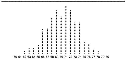
They refer to a common way that natural phenomena arrange themselves approximately. (The true normal distribution is a mathematical abstraction, never perfectly observed in nature.) If you look again at the distribution of high school boys that opened the discussion, you will see the makings of a bell curve. If we added several thousand more boys to it, the kinks and irregularities would smooth out, and it would actually get very close to a normal distribution. A perfect one is in the figure below.
A perfect bell curve
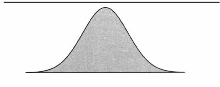
It makes sense that most things will be arranged in bell-shaped curves. Extremes tend to be rarer than the average. If that sounds like a tautology, it is only because bell curves are so common. Consider height again. Seven feet is “extreme” for humans. But if human height were distributed so that equal proportions of people were 5 feet, 6 feet, and 7 feet tall, the extreme would not be rarer than the average. It just so happens that the world hardly ever works that way.
Bell curves (or close approximations to them) are not only common in nature; they have a close mathematical affinity to the meaning of the standard deviation. In any true normal distribution, no matter whether the elements are the heights of basketball players, the diameters of screw heads, or the milk production of cows, 68.27 percent of all the cases fall in the interval between 1 standard deviation above the mean and 1 standard deviation below it. It is worth pausing a moment over this link between a relatively simple measure of spread in a distribution and the way things in everyday life vary, for it is one of nature’s more remarkable uniformities.
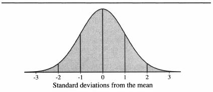
In its mathematical form, the normal distribution extends to infinity in both directions, never quite reaching the horizontal axis. But for practical purposes, when we are talking about populations of people, a normal distribution is about 6 standard deviations wide. The next figure shows how the bell curve looks, cut up into six regions, each marked by a standard deviation unit. The range within ±3 standard deviation units includes 99.7 percent of a population that is distributed normally.
A bell curve cut into standard deviations
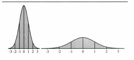
We can squeeze the axis and make it look narrow, or stretch it out and make it look wide, as shown in the following figure. Appearances notwithstanding, the mathematical shape is not really changing. The
standard deviation continues to chop off proportionately the same size chunks of the distribution in each case. And therein lies its value. The standard deviation has the same meaning no matter whether the distribution is tall and skinny or short and wide.
Standard deviations cut off the same portions of the population for any normal distribution
Furthermore, there are some simple characteristics about these scores that make them especially valuable. As you can see by looking at the figures above, it makes intuitive sense to think of a 1 standard deviation difference as “large,” a 2 standard deviation difference as “very large,” and a 3 standard deviation difference as “huge.” This is an easy metric to remember. Specifically, a person who is 1 standard deviation above the mean in IQ is at the 84th percentile. Two standard deviations above the mean puts him at the 98th percentile. Three standard deviations above the mean puts him at the 99.9th percentile. A person who is 1 standard deviation below the mean is at the 16th percentile. Two standard deviations below the mean puts him at the 2d percentile. Three standard deviations below the mean puts him at the 0.1th percentile.
Why go to all the trouble of computing standard scores? Most people understand percentiles already. Tell them that someone is at the 84th percentile, and they know right away what you mean. Tell them that he’s at the 99th percentile, and they know what that means. Aren’t we just introducing an unnecessary complication by talking about “standard scores”?
Thinking in terms of percentiles is convenient and has its legitimate
uses. We often speak in terms of percentiles—or centiles—in the text. But they can also be highly misleading, because they are artificially compressed at the tails of the distributions. It is a longer way from, say, the 98th centile to the 99th than from the 50th to the 51st. In a true normal distribution, the distance from the 99th centile to the 100th (or, similarly, from the 1st to the 0th) is infinite.
Consider two people who are at the 50th and 55th centiles in height. Using the NLSY as our estimate of the national American distribution of height, their actual height difference is only half an inch.
2
Consider another two people who are at the 94th and 99th centiles on height—the identical gap in terms of centiles. Their height difference is 3.1 inches, six times the height difference of those at the 50th and 55th centiles. The further out on the tail of the distribution you move, the more misleading centiles become.
Standard scores reflect these real differences much more accurately than do centiles. The people at the 50th and 55th centiles, only half an inch apart in real height, have standard scores of 0 and .13. Compare that difference of .13 standard deviation to the standard scores of those at the 94th and 99th centiles: 1.55 and 2.33, respectively. In standard scores, their difference—which is .78 standard deviation—is six times as large, reflecting the six-fold difference in inches.
The same logic applies to intelligence test scores, and it explains why they should be analyzed in terms of standard scores, not centiles. There is a lot of difference between people at the 1st centile and the 5th, or between those at the 95th and the 99th, much more than those at the 48th and the 52d. If you doubt this, ask a university teacher to compare the classroom performance of students with an SAT-Verbal of 600 and those with an SAT-Verbal of 800. Both are in the 99th centile of all 18-year-olds—but what a difference in verbal ability!
3