Understanding Sabermetrics (3 page)
Read Understanding Sabermetrics Online
Authors: Gabriel B. Costa,Michael R. Huber,John T. Saccoma

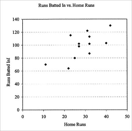
The data is entered point by point to create a picture called a
scatterplot
, and then we infer a curve or line that approximately passes through the points, which could then be used to predict second coordinates given a first coordinate. Here is the scatterplot for Hodges’ home run and runs batted in data:
scatterplot
, and then we infer a curve or line that approximately passes through the points, which could then be used to predict second coordinates given a first coordinate. Here is the scatterplot for Hodges’ home run and runs batted in data:
Figure 1.1 Scatterplot for Gil Hodges’ 12 seasons of HR and RBI
It would seem that a line having positive slope would pass through the points, which would indicate a positive correlation. Obviously, a straight line could not possibly hit every point. Figure 1.2 shows the scatterplot with line segments connecting up all the points.
If we wanted to find a line to model this data in order to make some predictions, we would find that every
x
-value in the data set has a
y
-value associated with it that would not actually lie exactly on a line. We want to find a line that best fits the data. One common method of finding such a line is a process leading to a line in which the data points are shown to have the minimum distance from it. Since the standard formula for distances involve square roots, a process in which the sum of the squares of the distances from the data points to their best fit line is called
the method of least squares
; the line is called
the least squares line
.
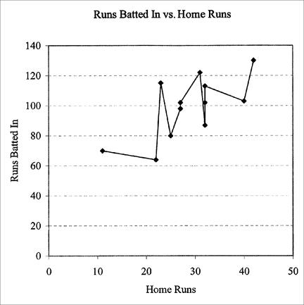
Figure 1.2 Scatterplot for Gil Hodges’ 12 seasons of HR and RBI, with line segments joining the points
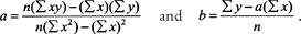
Recall that the slope-intercept equation for a line is generally represented as
y = mx + b
, where
x
represents the independent variable,
y
represents the dependent variable,
m
represents the
slope,
or the ratio of the difference between
y
-coordinates and the difference between their corresponding
x
-coordinates. The standard form for the least squares line is
y = ax + b,
where
For Gil Hodges’ home run and RBI data, these values are summarized in Table 1.2.
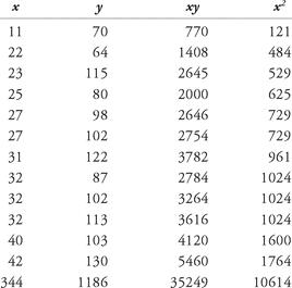
Table 1.2 Least squares computations for Gil Hodges’ 12 seasons
By the formulas,
a
= 1.66, and
b
= 51.21, so the regression line has equation
y
= 1.66
x
+ 51.21. Thus, if Hodges had hit 35 home runs in the season, he would be expected to have 1.66 × 35 + 51.21 RBI, or roughly 109, not “dead-on” perfect, but not unreasonable in the context of his other seasons. To determine just how good the fit is, we compute the correlation coefficient
r:
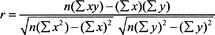
For this particular data set, the value of
r
is approximately 0.675. A value close to 1 indicates a high positive correlation, one close to -1 indicates a high negative correlation, and values close to zero mean a very weak correlation, or no correlation at all. Thus, Gil Hodges’ home runs are moderately correlated with his RBI.
r
is approximately 0.675. A value close to 1 indicates a high positive correlation, one close to -1 indicates a high negative correlation, and values close to zero mean a very weak correlation, or no correlation at all. Thus, Gil Hodges’ home runs are moderately correlated with his RBI.
Infield Practice: Sabermetrical Reasoning
Even though sabermetrics is defined as
the search for objective knowledge about baseball
, we must realize at the outset that the order of certainty in sabermetrics is nowhere near that of mathematics. To sabermetrically prove something means that a number of instruments (for example, runs created — see Inning 6: The Runs Created School) have been used to reinforce or strengthen a position, which, in turn, would make a conclusion plausible. But such a position should never be considered as permanently true as, for example, a proof of the Theorem of Pythagoras. There are just too many parameters and variables that Sabermetrics cannot take into account (see Seventh-Inning Stretch: Non-Sabermetrical Factors). In this chapter we illustrate how one might reason in a sabermetrical fashion, by way of an example which poses a number of questions which will be addressed throughout this book. We will not answer
all
the posed questions here; we will address them throughout the book as the relevant measures are presented.
In 1920, Babe Ruth hit 54 home runs, becoming the first player to slug thirty, forty and fifty home runs in a season. He also hit more home runs than every other American League team, and all but one of the National League clubs. A number of questions immediately arise:
• Was Ruth as dominant during any other year of his career?
• Did any of his contemporaries match his feat?
• Did any other slugger of any other era duplicate or surpass what Ruth did in 1920?
The first step is to look at the data. We see that, in addition to hitting such a heretofore unthinkable number of home runs, Ruth outdistanced the American League runner-up that season, fellow Hall of Famer George Sisler, by thirty-five home runs. Philadelphia Phillies’ center fielder, Cy Williams, led the National League in 1920 with fifteen homers. How significant were these differences? One way to address this question is to compare other seasonal home run champions with their runners-up; we will use this relativity technique in future discussions.
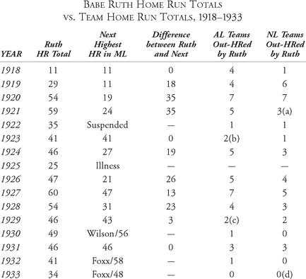
Table 2.1 Babe Ruth’s seasonal home run totals (1918-1933)
Back to Ruth, we also find that he actually out-homered
pairs
of major league teams. For example, in 1920 the St. Louis Cardinals and the Cincinnati Reds hit fifty home runs between the two clubs, falling four short of Ruth’s total. And there were ten other such pairs of teams that year. How significant was that? Did anybody else ever hit more home runs in a season than the combined total of two teams? If so, how many times? By all accounts, Ruth was a dominant force in 1920. Let us consider some other Ruthian years.
In Table 2.1, we consider sixteen of Babe Ruth’s seasons. We look at his home run totals, from 1918 through 1933. We put these numbers into the context of the major leagues during that time span, comparing Ruth to his runner-up and also looking at the number of teams Ruth out-homered, season by season. It should be noted that during this period, Ruth won or tied for twelve home run crowns. We also point out that Ruth was suspended for six weeks in 1922 for ignoring the prohibition against barnstorming ; this ban applied only to participants in the 1921 World Series. We note, too, that in 1925, Ruth spent a significant portion of the season out of the lineup due to illness. So, the Babe lost several games (or home run opportunities) during these two seasons. Finally, National Leaguer Hack Wilson led the major leagues with 56 home runs in 1930. Jimmie Foxx, of the American League, paced the major leagues in home runs during the 1932 and 1933 seasons.
a. Tied Brooklyn Dodgers in 1921
b. Tied Detroit Tigers in 1923
c. Tied St. Louis Browns in 1929
d. Tied Cincinnati Reds in 1933Note that Ruth won the AL home run title in 1930.
SUMMARY:
Ruth out-homered major-league teams 90 times, excluding 4 tiesRuth out-homered pairs of teams 18 times:1918 (1)
1920 (11)
1921 (3)
1927 (3)
So what can we make of this?
While much can be gleaned from this table, perhaps nothing is more telling than the dominance of Babe Ruth. We know
what
he did; in Sabermetrics, we ask “How can the significance of his performance over this sixteen-year period be measured?” Other questions follow, such as, “Was Ruth unique in what he accomplished?” Sabermetrical reasoning will assist us greatly in obtaining these answers. We give a table below which summarizes sabermetrical reasoning:
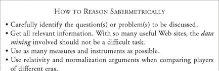
Figure 2.2 Sabermetrical reasoning
Other books
The Axe Factor: A Jimm Juree Mystery (Jimm Juree Mysteries) by Colin Cotterill
The Stalker by Bill Pronzini
The Marine's Naughty Sister by Terry Towers
The Sorcerer's Companion: A Guide to the Magical World of Harry Potter by Allan Zola Kronzek, Elizabeth Kronzek
Murder on Stage by Cora Harrison
The Chance You Won't Return by Annie Cardi
First Into Nagasaki by George Weller
Pathfinder Tales: Lord of Runes by Dave Gross
London Falling by T. A. Foster
After Forever Ends by Melodie Ramone