X and the City: Modeling Aspects of Urban Life (29 page)

There is a fundamental relationship between the flow of traffic
q
in vehicles per unit time, the concentration
k
in vehicles per unit distance, and the speed
u
of the traffic. It is
q
=
ku
. In general each of these quantities is a function of distance (
x
) and time (
t
), but the form
q
(
k
) =
ku
(
k
) may also be valuable. Another useful quantity is the spacing per vehicle,
s
=
k
⁻¹
. If
s
₀
is the minimum possible spacing, that is, when the vehicles are stationary (or almost so), then
is referred to as the
jam concentration
; but it has nothing to do with preservatives! Associated with the above “fundamental relationship”
q
=
ku
is, not surprisingly, a “fundamental diagram.” The overall features can be inferred as follows. When the concentration is zero, the flow must be zero, so
q
(0) = 0. Furthermore, the flow is
zero when
k
=
k
_j
, so
q
(
k
_j
) = 0. Since
q
≥ 0, ruling out the trivial case
q
≡ 0 there must be an absolute maximum
q
=
q
_max
somewhere in the interval (0,
k
_j
). This is obviously of interest to traffic engineers (and indirectly, to those in traffic).

There may be more than one relative maximum of course, but the case we’ll examine will have a single maximum—the “capacity” of the road.
Figure 10.1
shows a typical
q-k
diagram for this situation.

Suppose we take two measurements of the flow
q
(
x
,
t
) a short distance Δ
x
apart, at points
A
and
B
, respectively (traffic moving from
A
to
B
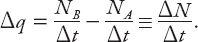
). The flow is defined to be the number of vehicles passing a given location in time Δ
t
; hence the change in
q
between the points
A
and
B
is given by

Within Δ
x
the change in the traffic density (or concentration)
k
is

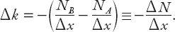
To see this, suppose without loss of generality that
N
_A
>
N
_B
, meaning that there is a build-up of cars between
A
and
B
, so the density in that spatial interval increases, that is, Δ
k
> 0, as indicated above in this case. It is assumed of course that there is no creation or loss of cars from within the interval (no white holes, sinkholes, or UFO abductions)—the total number of cars is constant. From these two equations for Δ
N
we see that

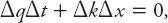
or

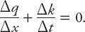
Now we invoke the continuum hypothesis (some shortcomings of which are discussed in
Chapter 15
and
Appendix 8
); we assume the quotients above possess well-defined limits as the discrete increments tend to zero, thus obtaining the limiting equation

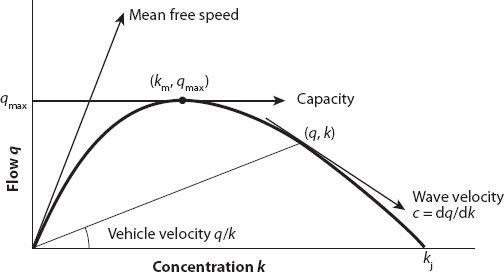
Figure 10.1. Flow-concentration diagram. The maximum is at the point of tangency (
k
_m
,
q
_max
).

This is the
equation of continuity
for the kinematic model. Note that it can be adapted to include the effects of entrances, exits and intersections, etc. by adding a term,
g
(
x
,
t
) say, to the right hand side. We will examine some simple consequences of equation (10.1); suppose that
q
=
q
(
k
); assuming the differentiability of
q
we have that

In the simplest possible case
dq
/
dk
=
c
, a constant, so the resulting equation is

This has the general solution