X and the City: Modeling Aspects of Urban Life (33 page)
Read X and the City: Modeling Aspects of Urban Life Online
Authors: John A. Adam

As above, this can be integrated, yielding

Again, we choose a steady-state traffic flow for which this reduces to

Since

we simplify this to the case when the traffic density is much less than the bumper-to-bumper density
k
max
= l/
l
(for which
u
= 0), that is,
k l/
l/
l
. Then (11.9) reduces to

upon which, as before, we impose the low density condition
u
=
u
max
to avoid singular behavior as
k
→ 0. The flow is therefore given by

For
u
to be continuous the choice of

must be made, but in this model the coefficient
B
has a more interesting interpretation. From equation (11.10) the maximum flow occurs when

and this occurs when
k
=
k
max
/e
. At this value of
k
, the speed of traffic is, from (11.10) simply
u
(
k
max
/e
) =
B
. For consistency with the continuity requirement,
k
c
must be such that

or more explicitly,


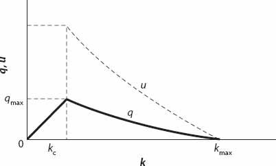
Figure 11.2.
q
(
k
) and
u
(
k
) profiles based on equations (11.11) and (11.10), respectively.
A generic sketch of both
u
(
k
) (dotted line) and
q
(
k
) is shown in
Figure 11.2
.
CAR FOLLOWING IN THE CITY—II

I love to watch clouds; their changing forms are indicative of the different kinds of hydrodynamical process that are present in the upper atmosphere, such as convection, shear flow, and turbulence. Unfortunately, I am rather prone to do this while driving. Probably the worst example of this occurred many years ago when my wife and I were on our way to the local hospital (she was in labor with our third child). I won’t elaborate here, except to say that she rightly urged me to concentrate on the road. Distractions such as cloud-watching while driving increase the reaction time for avoiding traffic hazards (and therefore should
not
be engaged in!). This next set of models incorporate reaction times in a simple and rather natural manner.
