X and the City: Modeling Aspects of Urban Life (30 page)

as is readily confirmed using the chain rule. In equation (10.4),
h
is a differentiable but otherwise arbitrary function. Its form depends on the so-called “initial conditions” at time
t
= 0 (say).

The solution (10.4) implies that
k
(and therefore
q
) travels to the right with “shape”
h
and speed
c
. If we recall that the mean speed of vehicles at a point is
u
=
q
/
k
then it follows that

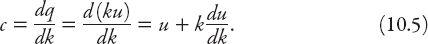
This is directly analogous to the relationship between the speed of individual waves in a medium and the speed of a group of them (a “wave packet”) in fluid dynamics. If
u
increases with traffic density (unlikely), then
c
>
u
, whereas if
u
decreases with
k
, the speed of the “wave”
c
<
u
. This gives some basic insight into traffic jams: although
u
is non-negative, a sufficiently negative value of
du
/
dk
can render
c
< 0; that is, changes in the traffic conditions propagate backward at speed |
c
|.

We may also infer some qualitative traffic behavior under the very reasonable assumption that the flow is in general a decreasing function of traffic density
k
. Now suppose that
k
decreases gradually in the forward direction, that is,
k
′(
x
) < 0. Then the front region of the flow moves out faster than the regions behind, the decrease in density is smeared out, and provided the range of
k
-values are less than
k
_m
(when
q
=
q
_max
), everything propagates in the forward direction. If this is not the case some of the traffic flow conditions may propagate backward.

By contrast, if there is a sharp decrease in
k
, such as at a traffic signal red light, the road behind the light will have a high density while that ahead will be empty of vehicles for some distance. The density behind is
k
=
k
_j
, the jam density, while that ahead is
k
= 0. Consequently there is an abrupt change when the light changes to green. We can think of this discontinuity as being a highly compressed collection of all possible
k
-values, which starts to “decompress” as traffic begins to flow. Each value of the density then propagates away at its own speed; those corresponding to
q
>
q
_max
travel backward, those for which
q
<
q
_max
travel forward, and since
c
=
q
′(
k
_m
) = 0 at
q
=
q
_max
, the latter do not move at all. Referring to
Figure 10.1
we see that the fastest forward speed corresponds to the tangent slope at
k
= 0 (a clear road ahead) and the fastest backward speed to that at
k
=
k
_j
. This is the rear boundary along which the traffic jam resolves.

At the traffic light,
k
=
k
_m
corresponding to capacity flow, since
q
′(
k
_m
) = 0. This means that a traffic signal is useful for determining the capacity flow by allowing jam conditions to build up before turning to green. If
R
is the duration of the red phase,
G
that of the green, and vehicles arrive at the light at a rate
q
_a
and leave at a rate
q
_l
, the total number of cars arriving in a complete cycle is
q
_a
(
R
+
G
). The condition for them all to pass through the junction during the succeeding green phase is
q
_a
(
R
+
G
) <
q
_l
G
. Therefore the capacity of the junction is given by the upper bound
Gq
_l
/(
R
+
G
).

If the density
k
increases with forward distance there will be a “pile-up” problem, because the flow is greater for lower concentrations. This results—hydrodynamically speaking—in a
shock wave
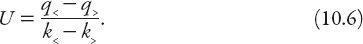
: a rapid transition from light traffic in the rear to heavy traffic in the front. No doubt we have all experienced this. Suppose that the set {
q
_>
,
k
_>
} describes the conditions just ahead of the shock front, and {
q
_<
,
k
_<
} behind it, and the shock moves at speed
U
. The rate at which vehicles emerge from the front of the shock wave is
q
_>
−
Uk
_>
; the rate at which they enter from the rear is
q
_<
−
Uk
_<
. The number of vehicles is conserved, so these rates are equal, so

This is the slope of the chord on the
q-k
diagram for a given
x
-value joining the shock wave entry and exit points. Note that in the limit as these differences tend to zero, the chord becomes the tangent line, and for that value of
x

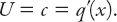
In summary, we have seen that according to the kinematic theory of traffic flow, the front of heavy traffic concentration tends to smooth out, whereas the rear steepens and forms a jam. A vehicle approaching from the rear encounters the heavy traffic suddenly, but exits it gradually. But we all know that from personal experience! And below we put a little more mathematical meat on those most annoying events, namely:

Let’s start this subsection off with a bang:

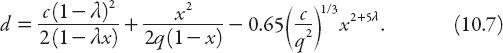
So there! What on earth does this formula mean? It is based on a model (Webster 1958) for the average delay per vehicle (
d
) at an intersection controlled by a traffic signal, and unfortunately it is too complicated to derive here. It was originally formulated for traffic in the UK and has been described as one of the most influential and useful results in this field of traffic control, known now as
the
Webster delay formula
, so we had better pay it some attention! The various parameters on the right-hand side of equation (10.7) are listed below:

It should be pointed out that the light sequence in the UK is red, red and amber (i.e., orange) together, green, amber, red, etc. The “effective green time” is (green + amber − 2) seconds, the 2 seconds being an allowance for delay in starting once the signal is green. The effective green time is easily adapted to the U.S. system in which the sequence is red, green, yellow, red, etc.

In equation (10.7) the first term represents the delay to the vehicles assuming a uniform arrival rate. The second term, a correction to the first, is the additional delay due to the randomness of vehicle arrivals. It is related to the probability that sudden surges in vehicle arrivals may cause temporary “oversaturation” of the signal operation. The third term, a subtractive one, is an empirical correction factor to correct the delay estimates consistent with observational data. It amounts to about 10% of the sum of the other terms. It is not surprising therefore that the following simplification to equation (10.7) is commonly used, namely,

Webster tabulated the delays (according to equation (10.7) for
s
using increments Δ
s
= 300 in the range [900, 3600]; for
c
(Δ
c
= 5) in the range [30, 60], and (Δ
c
= 10) in the range [60, 120]; for
q
(Δ
q
= 25) in the range [50, 1200] and for
g
(Δ
g
= 5) in the range [10, 100]. Let us calculate
d
from equation (10.8) for the values