X and the City: Modeling Aspects of Urban Life (9 page)

A representative diagram is shown in
Figure 3.8
.

I know that it’s usually a bad idea to go to the post office to mail letters when it first opens, especially on a Monday morning. And around the middle of December it’s a nightmare! But sometimes there is little or no line at all, even when the office is normally busy. That has happened on my last two visits. And conversely, sometimes there is a long line when I least expect it. While the average number of customers may be one every couple of minutes, it is most unlikely that each one will arrive every two minutes: there will be a certain “clumpiness” in the arrivals. The
Poisson distribution
describes this clumpiness well. Details and applications of this distribution are discussed in
Chapter 9
and in
Appendix 4
, but we will summarize the results here. If the arrivals at the post office, checkout line, traffic line, busstops, and so on are random and average to
λ
per minute (or other unit of time), then the probability
P
(
n
) of
n
customers arriving in any given minute is

Figure 3.8. Equidistance contours and “attraction” boundary for an elliptical city.

Suppose that on a reasonably busy day at the post office,
λ
= 2. What is the chance that there will be six customers ahead of me when I arrive? (Of course, there is also the question of how quickly on average the counter clerks serve the customers, but that is another issue.)

Then

or just over 1 percent. That’s not bad! And that’s just for starters; we will meet the Poisson distribution again in
Chapter 9
.

Another probability problem. Suppose that Jack and Jill, freshly arrived in the Big City, each have their own agendas about things to do. They decide—sort of—to do their “own thing” for most of the day and then meet sometime between 4:00 p.m. and 6:00 p.m. to have a bite to eat and discuss the day’s activities. Both of them are somewhat disorganized, and they fail to be more specific than that (after all, there are
so
many books to look at in Barnes and Noble, or Foyle’s Bookshop in London, who knows when Jack will be ready to leave?) Furthermore, neither cell (mobile) phone is charged, so they cannot ask “where the heck are you?”

Suppose that each of them shows up at a random time in the two-hour period. Jack is only willing to wait for 15 minutes, but Jill, being the more patient of the two (and frankly, a nicer person) is prepared to wait for half an hour. What is the probability they will actually meet? The related question of what will happen if they don’t is beyond the scope of this book, but the first place to start looking might be the local hospital.

This is an example of geometric probability. In the 2-hr square shown in
Figure 3.9
, the diagonal corresponds to Jack and Jill arriving at the same time at any point in the 2-hr interval. The shaded area around the diagonal represents the “tolerance” around that time, so the probability that they meet is the ratio of the shaded area to the area of the square, namely,

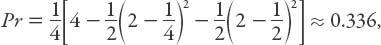
or about one third. Not bad. Let’s hope it works out for them.

To build housing requires land (
L
) and materials (
M
), and if the latter consists of everything that is not land (bricks, wood, wiring, etc.), then we can define a function
Q
(
L
,
M
),

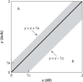
Figure 3.9. The shaded area relative to that of the square is the probability that Jack and Jill meet.

where
a
> 0 and 0 ≤
λ
≤ 1. This form of function is known as a
Cobb-Douglas
production function, widely used in economics, and named for the mathematician and U.S. senator who developed the concept in the late 1920s.

If the price of a unit of housing is
p
, the cost of a unit of land per unit area is
l
, and the cost of unit materials is
m
(however all these units may be defined), then the builders’ total profit
P
is given by

If a speculative builder wishes to “manipulate”
L
and
M
to maximize profit, then at a stationary point

Exercise:
(i) Show, using equation (3.16), that this set of equations takes the algebraic form

(ii) Show also from equation (3.16) that according to this model, such a speculator “gets his just deserts” (i.e.,
P
= 0)!