Understanding Sabermetrics (11 page)
Read Understanding Sabermetrics Online
Authors: Gabriel B. Costa,Michael R. Huber,John T. Saccoma

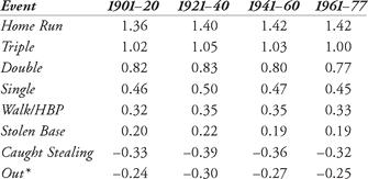
Table 6.1 Palmer’s run values of various events, by periods
In his chart, Palmer noted that “an out is considered to be a hitless at-bat and its value set so that the sum of all events times their frequency is zero, thus establishing zero as the base line, or norm, for performance.” A few years after Palmer published his study, statistician Dave Smith (of
Retrosheet
) suggested to Palmer that he might adjust the coefficients for stolen base and caught stealing events, as they were situation dependent. In a 1980 article entitled, “Maury Wills and the Value of a Stolen Base,” Smith wrote that players elected to steal bases, and stolen bases were attempted more frequently in close baseball games. Palmer accepted the advice and revised his coefficients to be 0.30 and - 0.60, respectively.
John Thorn then teamed with Pete Palmer to develop the Linear Weights model for predicting runs produced by a batter. They published The Hidden Game of Baseball in 1984. Their new model took an in-depth view into scoring runs. Run values evolved as playing conditions changed, and the two authors also wrote that run values depend on the batting order and batting position. Traditional leadoff batters are not power hitters, so a home run is not worth as much to them as to a clean-up batter. The 1984 linear-weights formula for batting runs is
Batting Runs = (0.46 × 1B) + (0.80 × 2B) + (1.02 × 3B) + (1.40 × HR) + [0.33 × (BB + HBP)] + (0.30 × SB) - (0.60 × CS) - [0.25 × (AB - H)] - (0.50 × OOB)
According to the linear-weights model, a home run is worth, on average, 1.40 runs over the course of an average season, while getting caught stealing loses a hitter 0.60 runs. The last term in this formula is an effort to take outs from plate appearances into account; subtracting hits and walks from plate appearances gives outs, and this term received a negative run weight. According to Thorn and Palmer, “while a single or walk always has a potential run value, a long fly does not unless a man happens to be posed at third base.” When this formula was first revealed, statisticians expected to see events such as sacrifices, sacrifice hits, grounded into double plays, and reached on error. Notice also that the coefficients for 1B, 2B, 3B, and HR are very close to those proposed by both Lane’s second model and Lindsey’s model. Further, Thorn and Palmer postulated that a home run was only worth about three times as much as a single, which is close to a half run less than suggested by Lindsey’s formula. In fact, they omit the stealing, caught stealing and outs-on-base terms when comparing the great players of the past, as data for caught stealing is not known. They thus used a condensed form for linear weights, given by:
Batting Runs = (0.47 × 1B) + (0.78 × 2B) + (1.09 × 3B) + (1.40 × HR) + [0.33 × (BB + HBP)] - [0.25 × (AB - H)]
Notice that the value of a single is 0.47 runs, and each extra-base hit (double, triple, home run) has a value of 0.31 times the number of bases beyond a single. They claim that this condensed version is accurate to within a fraction of a run.
How effective is the Linear Weights model? First, we mention that, just as with George Lindsey’s run model, Thorn and Palmer’s linear-weights model is a deviation from average performance. A batter with a positive linear-weights run production is above the average player, while a batter with a negative run production would be below average. Let’s consider a comparison of selected players from the 1960s. Table 6.2 shows a listing of all of the players (non-pitchers) who won the Most Valuable Player Award from 1960 through 1969 in both the National and American Leagues. In the columns next to their names are the seasons in which each won the league MVP award. We then list the seasonal offensive data and the linear-weights-model run production (LW Runs, using the condensed formula).
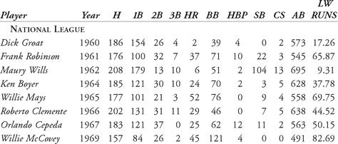

Table 6.2 Linear weights batting runs for MVPs from 1960 to 1969
From Table 6.2, we notice that Willie McCovey’s 1969 MVP season with the San Francisco Giants led to a batting run production of 82.69 runs above average. Dick Groat, on the other hand, won the 1960 Most Valuable Player Award with a run production of only 17.26 runs. When Maury Wills’ 104 stolen bases are taken away, his run production fell to 9.31 total batting runs. All of the batters listed were “above average,” but some were notably more than others. Despite only 377 official at-bats in 1962, the American League’s MVP, Mickey Mantle, still produced 66 more runs than the average player, according to the linear-weights model. Compare his production to his 1962 National League counterpart, Maury Wills. Wills had over 300 more at-bats, 87 more hits, and 95 more stolen bases, yet his run production is a fraction of Mantle’s.
Let’s compare the 1962 seasons of Mantle and Wills using more traditional statistics. Mantle’s batting average in 1962 was 0.321; his on-base percentage was 0.486, and his slugging percentage was a respectable 0.605. He had 228 total bases. Wills, in comparison, had a 0.299 batting average, 0.347 on-base percentage, and 0.373 slugging percentage, accounting for 259 total bases. Wills’ stolen bases accounted for 77 percent of his run production. Mantle’s nine stolen bases accounted for about 4 percent of his total runs. However, Mantle’s 30 home runs and 123 walks and HBP dwarf Wills’ six home runs and 53 walks and HBP. Without the stolen bases, Wills does not appear to have contributed many runs above the average.
In 1984, Thorn and Palmer mentioned that their linear-weights statistics have a “shadow stat which tracks its accuracy to a remarkable degree and is a breeze to calculate: OPS, or On Base Average Plus Slugging Percentage.” They went on to mention that the correlation between linear weights and OPS over the course of an average team’s regular season was 99.7 percent. OPS has since become a fixture in measuring the offensive production of a player. The linear-weights model is just as insightful. In 1962, Mantle’s OPS was 0.321 + 0.605 = 0.926. Wills, by comparison, had an OPS of 0.299 + 0.373 = 0.672, or 0.254 points lower. High OPS correlates to producing more runs above average for a batter’s team. However, since OPS is not expressed in terms of runs, Thorn and Palmer felt that it was a less versatile statistic than their linear-weights. They explained that run scoring for teams is proportional to the on-base average times the slugging percentage (also known as the SLOB), while runs produced by a batter in an average lineup are proportional to his on-base average plus slugging percentage (OPS).
The linear weights batting run-production model seeks to assign run values to each offensive play. Certain events are not accounted for, however. As mentioned earlier, it does not predict runs based on sacrifices, sacrifice flies, grounded into double plays, or plays in which the batter reached on an error.
Pete Palmer published another article in the inaugural issue (1982) of
The National Pastime: A Review of Baseball History
. Palmer was chairman of SABR’s statistical analysis committee and John Thorn was the editor of
The National Pastime
. In an article entitled, “Runs and Wins,” Palmer expanded on a notion which he felt had received little attention to that point: the relationship of runs scored and allowed to wins and losses. He was interested in “how many games a team ought to have won, how many it did win, and which teams’ actual won-lost records varied far from their probable won-lost records.” In this article, Palmer cites earlier work by Earnshaw Cook. In 1964, Cook published
Percentage Baseball
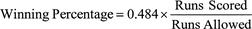
, which examined major league results from 1950 through 1960. In that paper, Cook determined that the winning percentage of a team was given by the following formula:
The National Pastime: A Review of Baseball History
. Palmer was chairman of SABR’s statistical analysis committee and John Thorn was the editor of
The National Pastime
. In an article entitled, “Runs and Wins,” Palmer expanded on a notion which he felt had received little attention to that point: the relationship of runs scored and allowed to wins and losses. He was interested in “how many games a team ought to have won, how many it did win, and which teams’ actual won-lost records varied far from their probable won-lost records.” In this article, Palmer cites earlier work by Earnshaw Cook. In 1964, Cook published
Percentage Baseball
, which examined major league results from 1950 through 1960. In that paper, Cook determined that the winning percentage of a team was given by the following formula:
The example provided in the paper cites the 1965 Minnesota Twins, who scored 774 runs while yielding 600. Their winning percentage should have been 0.484 times 774 divided by 600, or 0.630. The ’65 Twins, in fact, finished the season with 102 wins and 60 losses, for a winning percentage of 0.623. In “Runs and Wins,” Palmer states that his work showed that, “as a rough rule of thumb, each additional ten runs scored (or ten less runs allowed) produced one extra win.” He also found that high-scoring teams needed more runs to produce a win. Interestingly, he determined the exact run-per-win factor for an individual team to be equal to ten times the square root of the actual number of runs scored per inning by both teams. So, if two average teams both score 4.5 runs in a game, that is one total run per inning. Taking the square root of one and multiplying by ten yields a run-per-win factor of ten. This means that, using Lindsey’s model, Ty Cobb would have personally contributed over 14 wins to his 1911 Tigers team. Using linear weights, Cobb produced 107.33 runs (caught stealing statistics are not available for that season), which converts to about 11 wins, still a very impressive total.
Let’s revisit the Most Valuable Players from the 1960s. Using Palmer’s run-per-win factor of ten, we see that Willie McCovey contributed more than 8 wins above average (WAA) for his Giants squad, while teammate Willie Mays contributed seven WAA for his 1965 Giants team. Frank Robinson had seven WAA for each of his teams, the 1961 Reds and the 1966 Orioles; Carl Yastrzemski produced seven WAA for the 1967 Red Sox, and Harmon Killebrew has 7.5 WAA for his 1969 Twins. It’s interesting that Dick Groat won the 1960 Most Valuable Player Award in the National League by contributing only about one and a half WAA to the Pirates. Groat won the MVP by a landslide vote, garnering 16 of 22 first-place votes. However, his Pittsburgh teammates were well represented in the balloting; Don Hoak finished second, Cy Young Award winner Vern Law finished tied for sixth, Roberto Clemente finished eighth, Roy Face finished twelfth, and Smoky Burgess finished tied for twentieth (see the “Easy Tosses” at the end of the chapter to determine the linear weights runs for Groat’s teammates in 1960).
Other books
Towards Another Summer by Janet Frame
Las sandalias del pescador by Morris West
An Unsuitable Duchess by Laurie Benson
Slated for Death by Elizabeth J. Duncan
Christmas Showdown by Mackenzie McKade
MB02 - A Noble Groom by Jody Hedlund
Ironhand's Daughter by David Gemmell
2 Dead & Buried by Leighann Dobbs
Malice's Possession by Jenika Snow
Mud and Gold by Shayne Parkinson