Nonplussed! (3 page)

Figure 1.3.
P
(0,0) plotted against
p
.

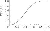
Figure 1.4.
P
(30,15) plotted against
p
.

Figure 1.5.
P
(40,30) plotted against
p
.

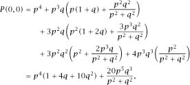
and so we have found the second of our expressions

We only need the starting probability
P
(0,0), which is by far the hardest goal, and to reach it without getting lost we will make use of the more complex tree diagram in
figure 1.2
, which again
shows the ways in which the situations divide until a known probability is reached. We then have

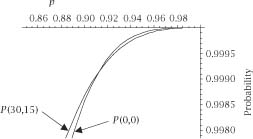
Figure 1.6.
The intersection of
P
(0,0) with
P
(30,15).

and the final expression needed is

Plots of the three probabilities, shown in
figures 1.3
–
1.5
, for all values of
p
(remembering that
q
= 1 −
p
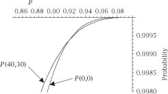
) show that they have very similar behaviour to one another, but there are intersections and if we plot the pairs
{P(
0,0
),P(
30,15
)}
and
{P(
0,0
),P(
40,30
)}
on the same axes for large
p
we can see them. This is accomplished in
figures 1.6
and
1.7
.

Of course, to find those intersections we need to do some algebra.

Figure 1.7.
The intersection of
P
(0,0) with
P
(40,30).

The Intersection of P(
30,15
) and P(
0,0)

To find the point of intersection we need to solve the formidable equation

again remembering that
q
= 1 −
p
.

Patience (or good mathematical software) leads to the equation in
p
,

which has repeated trivial roots of
p
= 0,1 as well as the roots of the quadratic equation 8
p
²
− 4
p -
3 = 0.

The only positive root is
and for any
p
> 0.911 437 … we will have
P
(0,0
) > P(
30,15) and the result for this case is established.

The Intersection of P(
40,30
) and P(
0,0)

This time the equation to be solved is

and, after a similarly extravagant dose of algebra, this reduces to

which again has trivial roots of
p
= 0,1.