X and the City: Modeling Aspects of Urban Life (81 page)
Read X and the City: Modeling Aspects of Urban Life Online
Authors: John A. Adam

Figure A7.1. Geometry of the probability of a point
P
being in the annular region.
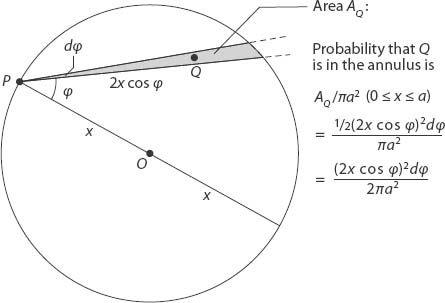
Figure A7.2. Probability of a point
Q
being in the (approximately) triangular sector.

We also need to know the average distance between
P
and
Q
in this sector; a simple “center of mass” argument will suffice here—it lies 2/3 of the way from the “base” of the triangular sector, so the average distance is 4
x
(cos )/3. Combining all these results gives expected distance between the two random points
P
and
Q
:

There is an additional factor of two in this integral to include the case when
P
is nearer to the center than
Q
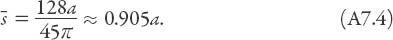
. This integral can be evaluated by careful calculus students to be
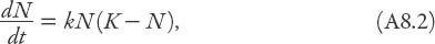
INFORMAL “DERIVATION” OF THE LOGISTIC
DIFFERENTIAL EQUATION
It has been said that there are two categories of people in the world: those that separate people into two categories and those that don’t. Nevertheless, suppose there are indeed two categories of people (described below) comprising a community: in which the population is constant. This may seem very unrealistic, except over short periods of time, for what about births, deaths, “emigration,” and “immigration” within such a community? And while this is a valid criticism, there are several “communities” that possess a constant population: cruise liners, and political bodies (House, Senate, etc.) being two such examples. We shall examine the mathematical genesis of the logistic equation in the former context, but not before identifying a limitation inherent in this approach. A cruise liner may have a thousand passengers (and several hundred crew members) on board, whereas the United States Senate has one hundred members. In each case, the total population is constant (ignoring people falling overboard in the former case, of course!), but within each community, there may be two classes of subpopulations. Obviously the number of males and females remains fixed, so what could vary?
We’ll make some simplifying assumptions here. Suppose that a passenger with a contagious and easily transferable disease boards the cruise liner (without exhibiting any symptoms at that time). Over time, assuming all the other passengers are susceptible to this disease, as the infected individual comes into contact with them, the number of infected passengers increases—and this is certainly something that has happened on several occasions in recent years. So in this case, at any given time in this simplified model, there are two categories of passengers: those who are infected and those who are not. And in this model these populations will vary monotonically over time subject only to the
condition that their sum is a constant,
K
. We could change the scenario from transference of a disease to that of a rumor: gossip! In that case there would be additional assumptions to be made: everyone who knew the rumor would be willing to share it, and everyone who did not know it would be willing to listen (and hence pass it on!). A related context is that of advertising by word of mouth: “Did you hear about the special offer being made at Sunbucks? They’re giving away a Caribbean cruise to everyone who buys a Grande peppered Latvian pineapple-cauliflower espresso mocha latté.”
In the case of the U.S. Senate, suppose that Senator A introduces a bill (maybe to restrict the availability of the above coffee at Sunbucks because of its harmful effects on the local populace?). Perhaps there is little support for the bill initially (many of the senators like that coffee), and as acrimonious but eloquent debate continues, more and more senators begin to see the error of their ways, and eventually vote accordingly. . . . Again, there will be an evolution of the potential “Aye” and “Nay” votes over time, culminating in, well, you’ll just have to tune in to C-Span to see the outcome.
So what is the limitation of this approach, regardless of context? Nothing yet, but if we use calculus to try to describe the rate of change of the two populations, we are making the implicit assumption of differentiability, and hence continuity of the populations. But the populations are discrete! The are always an integral number of infected passengers, or of senators disposed to vote for the bill (and despite one’s personal misgivings about Senator B, though he may only do the work of half a senator, he is one person). Calculus is strictly valid when there is a continuum of values for the variables concerned, and in that sense calculus-based models of discrete systems can never be totally realistic, even when there are billions of individuals (such as the number of cells in a tumor). It is usually the case in practice that the more individuals there are in a population, the more appropriate the mathematical description will be from a continuum perspective, because small populations can be subject to fluctuations that are comparable in size with the population! Under those circumstances a discrete approach is desirable. Nevertheless, when the number of possible “states” is limited (as in “Aye” or “Nay,” infected or not), frequently the calculus-based approach is sufficiently accurate to “interpolate” the behavior of the more accurate discrete formulation. And that is what we shall do here in the context of the cruise liner epidemic, neglecting all complications like incubation times, likelihood of recovery, and immunity from the disease.
Such considerations are very important in realistic epidemiological models, but will not be addressed here. We are therefore assuming that all passengers who are uninfected at the beginning of the cruise are susceptible to the disease, and that once they have contracted it, they remain infected (and infectious) for the duration of the cruise (a very unfortunate scenario). The problem then becomes one of determining how the number of passengers contracting the disease changes over time. Let
N
(
t
) be the number of infected passengers and
M
(
t
) be the number not infected. Obviously
M
(
t
) +
N
(
t
) =
K
and, as stated above,
N
(0) = 1 (this initial condition can be changed without loss of generality). Remembering that the argument we are making here is not a rigorous one, let us take two such passengers at random, and ask what the probability of the spread of the disease will be from such an encounter. Certainly, the only way the disease will spread is if each of these two individuals is in a different category. To reframe this in the “rumor” category, if our two individuals know of the rumor, then to begin with, they may just talk about the weather (especially if they are from the UK!); if both know the rumor, they may just talk about . . . the weather. It is only when one of the two knows the rumor, and the other does not, that the rumor will spread. And so it is with the disease under the simplifying assumptions we have made. The probability of picking an individual from the infected population and then one from the uninfected is

so the probability of the infection spreading from this encounter is proportional to
NM
, and this is just
N
(
K
−
N
). Furthermore, it is reasonable to suppose that the rate of change of
N
is proportional to this probability, that is,