Nonplussed! (27 page)

gives

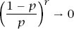
and so the equation of the spiral becomes

and the solution path to the problem is

This spiral must at some time cross the smuggler’s path and when it does the two ships will be equidistant from
P
₁
, as shown in
figure 10.8
, and so they will be in the same place. Capture is certain!

If the smuggler’s track makes an angle
with the positive
x
-direction, the capture will take place when
(where
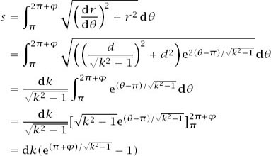
) and so we can calculate the distance travelled to interception by calculating the arc length of the path from
θ
=
π
to
, which we can deduce from the second form of the result from appendix C,

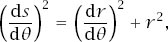
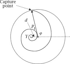
Figure 10.8.
Captured!

to get

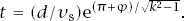
and the time to interception is given by

where
. This means that

PARRONDO’S GAMES

This is a one line proof… if we start sufficiently far to the left.

Unknown Cambridge University lecturer

We are all used to the idea of losing in any number of games of chance, particularly in games which are biased against us. If we decide to alleviate the monotony of giving our money away by varying play between two such games, we would reasonably expect no surprises in the inevitability of our financial decline, but that is to ignore the discovery of Dr Juan Parrondo:
two losing games can combine to a winning composite game
.

We will avoid the rigorous definition of a losing game since we all have an instinctive feel for what one is, and that is enough for our purposes; in short, if we are foolish to gamble on such a game, in the long term we expect to finish up with less money than we started with. Put more mathematically, the probability of our winning on any play of the game is less than 0.5. (We can also lose even if it equals 0.5 if our wealth is small compared with the other player; the reader may wish to investigate the implications of what is known as
gambler’s ruin
.) Now suppose that there are two such games, call them A and B, which we might
play individually or in combination, with the pattern for playing the combination quite arbitrary: we could play A for a while and then change and continue gambling by playing B, or we could alternate playing ABABAB … or toss a (possibly biased) coin to determine which we play and when, etc. Whatever the strategy we use to decide which game to play and when, we would expect to lose in the long term, but the force of Parrondo’s result is that situations exist which result in a winning combination. The public announcement was made (in particular) in the 1999 article, ‘Parrondo’s Paradox’, by G. P. Harmer and D. Abbott in
Statistical Science
14(2):206–13. Three years earlier the Spanish physicist Juan M. R. Parrondo had presented the idea in unpublished form at a workshop in Turin, Italy: he had defined a composite, winning game from two provably losing games; that is, the player’s fortune provably increases as he continues to play the combined game. It is this process which attracts our attention in this chapter, as we look at
Parrondo’s Games
.

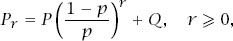
The Basic Game

The study is part of the much bigger topic of Markov chains, but here we need the simplest of ideas from them. Suppose that we repeatedly play a game and either win 1 unit with a constant probability
p
or lose 1 unit with probability 1 −
p
. We will start with some fortune and write
P
_r
for the probability that our fortune is reduced to 0 when it is currently at a level
r
; we will not consider the possibility of exhausting the wealth of our opponent.

Figure 11.1
summarizes the position as we take one more gamble, which means that

and also we clearly have that
P
₀
= 1.

This summarizes such a game and provides us with what is known as a recurrence relation for the
P
_r
; what we would like is an explicit expression for
P
_r
in terms of
p
and
r
.

Figure 11.1.
The basic tree diagram.

The trick that accomplishes this is to try a solution of the form
P
_r
=
x
^r
, which results in

and cancelling by
x
^r
−1
results in
x
=
px
²
+ (1 −
p
) or

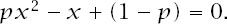
This quadratic equation factorizes to (
x
− 1)(
px
− (1 −
p
)) = 0 and so has roots
x
= 1 and
x
= (1 −
p
)/
p
. This means that

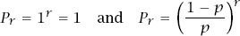
are both solutions, which we can easily check by substituting each of them in equation (1).

This isn’t the full story, though. Again, it is easy to check that any constant multiple of each solution is again a solution, and, further, that the sum of each of the two solutions is itself a solution. This results in the completely general solution of (1) of

for constants
P
and
Q
.

We can now invoke the condition that
p
₀
= 1 to get
P
+
Q
= 1, which provides us with one equation in two unknowns and to find unique values of
p
and
Q
we need a second, independent equation. This is not quite so easy.

If the opponent had a known capital, which would allow us to write the total initial capital between the two players as, say,
N
, we could also invoke the condition
PN
= 0, which would result in that second equation for
p
and
Q
and this would mean that the values could be established. As it is, we have no such condition, but we can make progress by using the following intuitive argument.

It must be that (1 −
p
)/
p
is equal to, greater than or less than 1, and we can consider the three cases separately.

If (
1
−
p
)/
p
= 1 (that is,
), then
P
_r
=
P
+
Q
= 1 and in the long term we are assured of losing all of the capital against an opponent of much greater wealth.

If (1−
p
)/
p
> 1, as
r
increases
P
_r
is bound to fall outside [0, 1] and so violate the laws of probability, that is, unless
P
= 0, which makes
P
_r
= 1 for all
r
.

Now suppose that (1 −
p
)/
p
< 1, then, as
r
increases,